สารบัญ

APPENDIX 9 STATISTICAL ANALYSIS OF RESULTS OF BIOLOGICAL ASSAYS AND TESTS

1. Introduction 

          This appendix provides guidance for the design of biological assays prescribed in the Thai pharmacopoeia and for analysis of their results. It is intended for use by those whose primary training and responsibilities are not in statistics, but who have responsibility for analysis or interpretation of the results of these assays, often without the help and advice of a statistician. The methods of calculation described in this appendix are not mandatory for the biological assays which themselves constitute a mandatory part of the Thai Pharmacopoeia. Alternative methods may be used, provided that they are not less reliable than those described here. A wide range of computer software is available and may be useful depending on the facilities available to, and the expertise of, the analyst.

          Professional advice should be obtained in situations where: a comprehensive treatment of design and analysis suitable for research or development of new products is required; the restrictions imposed on the assay design by this appendix are not satisfied (for example, particular laboratory constraints may require customized assay designs, or equal numbers of equally spaced doses may not be suitable); analysis is required for extended non-linear doseresponse curves (for example, as may be encountered in immunoassays). An outline of extended dose-response curve analysis for one widely used model is nevertheless included and a simple example is given (See Section 3.1.4).

GENERAL DESIGN AND PRECISION

          Biological methods are described for the assay of certain substances and preparations whose potency cannot be adequately assured by chemical or physical analysis. The principle applied wherever possible throughout these assays is that of comparison with a standard preparation so as to determine how much of the substance to be examined produces the same biological effect as a given quantity, the Unit, of the standard preparation. It is an essential condition of such methods of biological assay that the tests on the standard preparation and on the substance to be examined be carried out at the same time and under identical conditions.

          For certain assays (determination of virus titre for example) the potency of the test sample is not expressed relative to a standard. This type of assay is dealt with in Section 3.2.4.

          Any estimate of potency derived from a biological assay is subject to random error due to the inherent variability of biological responses and calculations of error should be made, if possible, from the results of each assay, even when the official method of assay is used. Methods for the design of assays and the calculation of their errors are, therefore, described below. In every case, before a statistical method is adopted, a preliminary test is to be carried out with an appropriate number of assays, in order to ascertain the applicability of this method.

          Estimates of error are themselves subject to appreciable error if they are not based on a very large number of observations. The calculations may thus lead to false conclusions unless some allowance is made for this fact, as may be done by the calculation of fiducial limits. Since most of the responses to the biological assays are normally distributed, the fiducial limits are therefore replaced by the confidence limits.

          The confidence interval for the potency gives an indication of the precision with which the potency has been estimated in the assay. It is calculated with due regard to the experimental design and the sample size. The 95 per cent confidence interval is usually chosen in biological assays. Mathematical statistical methods are used to calculate these limits so as to warrant the statement that there is a 95 per cent probability that these limits include the true potency. Whether this precision is acceptable to the Thai Pharmacopoeia depends on the requirements set in the monograph for the preparation concerned.

          The following terms are used in this appendix to indicate the corresponding concepts:

 

Term	Definition
Stated potency	A nominal value assigned from knowledge of the potency of the bulk material, in the case of a formulated product; the potency estimated by the manufacturer, in the case of bulk material.
Labelled potency	The same as stated potency.
Assigned potency	The potency of the standard preparation.
Assumed potency	The provisionally assigned potency of a preparation to be examined which forms the basis of calculating the doses that would be equipotent with the doses to be used of the standard preparation.
Potency ratio of an unknown preparation	The ratio of equipotent doses of the standard preparation and the unknown preparation under the conditions of the assay
Estimated potency	The potency calculated from assay data.
Experimental unit	A subject or a set of subjects, received a treatment at a time.

          Glossary of symbols is a tabulation of the more important uses of symbols throughout this appendix (See Section

6). Where the text refers to a symbol or uses a symbol to denote a different concept, this is defined in that part of the text.

2. Randomization and Independence of Individual Treatments

          The allocation of the different treatments to different experimental units (animals, tubes, etc.) should be made by some strictly random process. Any other choice of experimental conditions that is not deliberately allowed for in the experimental design should also be made randomly. Examples are the choice of positions for cages in a laboratory and the order in which treatments are administered. In particular, a group of animals receiving the same dose of any preparation should not be treated together (at the same time or in the same position) unless there is strong evidence that the relevant source of variation (for example, between times, or between positions) is negligible. Random allocations may be obtained from computers by using the built-in randomization function. The analyst must check whether a different series of numbers is produced every time the function is started.

          The preparations allocated to each experimental unit should be as independent as possible. Within each experimental group, the dilutions allocated to each treatment are not normally divisions of the same dose, but should be prepared individually. Without this precaution, the variability inherent in the preparation will not be fully represented in the experimental error variance. The result will be an underestimation of the residual error leading to:

          1) an unjustified increase in the stringency of the test for the analysis of variance.

          2) an underestimation of the true confidence limits for the test which are calculated from the estimate of s² , the residual error mean square.

3. Assay Design and Analysis

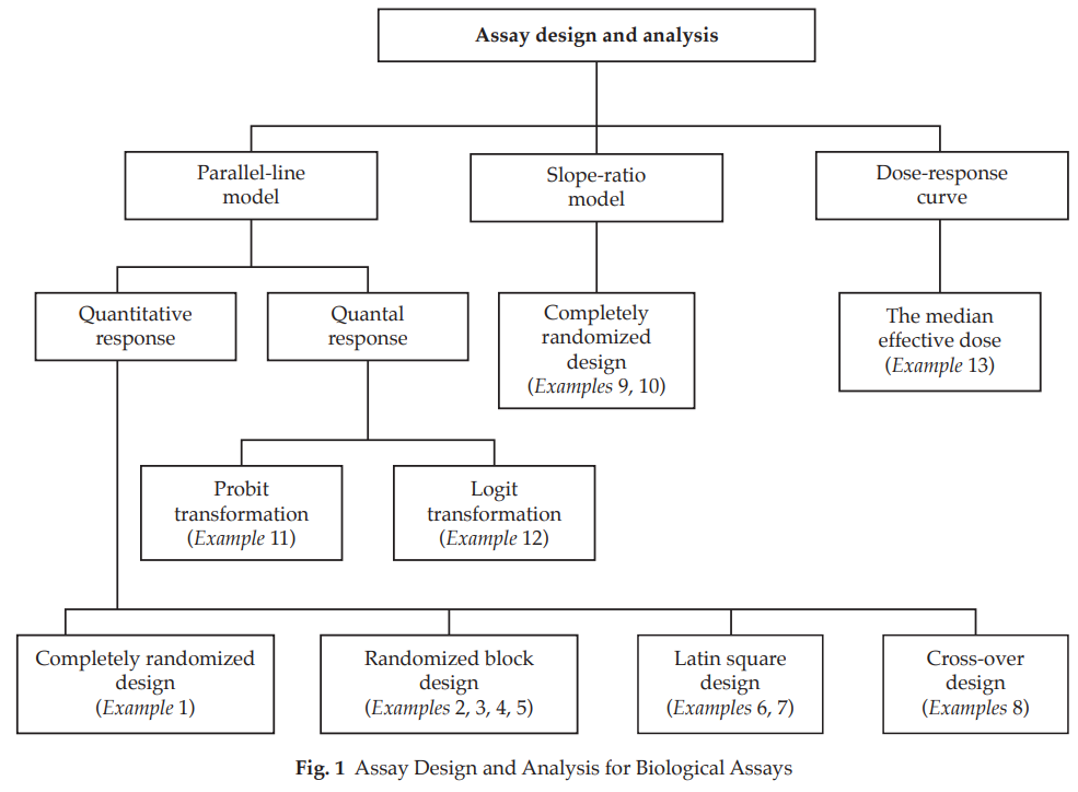
          Numerous assay designs and analyses described herein (Fig. 1) can be chosen under certain conditions. There are three types of assays: the parallel-line model, the slope-ratio model, and the dose-response curve. The biological responses may be quantitative or quantal. Quantitative responses are the measurement of the effect on each experimental unit on a quantitative scale and quantal responses are on a qualitative scale. Under the parallel-line model with quantitative responses, there are four assay designs prescribed: the completely randomized design, the randomized block design, the Latin square design and the cross-over design. For the quantal response of parallelline model, the probit and logit transformations are performed. The design used in the slope-ratio model is the completely randomized design, and the median effective dose is shown for the dose-response curve.

3.1 ASSAYS DEPENDING UPON QUANTITATIVE RESPONSES

         3.1.1 Statistical models​

         3.1.1.1 General principles

         The biological assays included in the Thai Pharmacopoeia have been conceived as “dilution assays”, which means that the unknown preparation to be assayed is supposed to contain the same active principle as the standard preparation, but in a different ratio of active and inert components. In such a case the unknown preparation may in theory be derived from the standard preparation by dilution with inert components. To check whether any particular assay may be regarded as a dilution assay, it is necessary to compare the dose-response relationships of the standard and unknown preparations. If these dose-response relationships differ significantly, then the theoretical dilution assay model is not valid. Significant differences in the dose-response relationships for the standard and unknown preparations may suggest that one of the preparations contains, in addition to the active principle, other components which are not inert but which influence the measured responses.

         To make the effect of dilution in the theoretical model apparent, it is useful to transform the dose-response relationship to a linear function on the widest possible range of doses. Two statistical models are of interest as models for the biological assays prescribed: the parallel-line model and the slope-ratio model.

         The application of either is dependent on the fulfillment of the following conditions:

Condition 1: the different treatments have been randomly assigned to the experimental units,

Condition 2: the responses to each treatment are normally distributed,

Condition 3: the standard deviations of the responses within each treatment group of both standard and unknown preparations do not differ significantly from one another.

         When an assay is being developed for use, the analyst has to determine that the data collected from many assays meet these theoretical conditions.

---- Condition 1 can be fulfilled by an efficient use of Section 2.

---- Condition 2 is an assumption which in practice is almost always fulfilled. Minor deviations from this assumption will in general not introduce serious flaws in the analysis as long as several

replicates per treatment are included. In case of doubt, a test for deviations from normality (e.g., the Shapiro-Wilk test¹ ) may be performed.

---- Condition 3 can be checked with a test for homogeneity of variances (e.g., Bartlett’s test² , Cochran’s test³ ). Inspection of graphical representations of the data can also be very instructive

for this purpose.

When conditions 2 and/or 3 are not met, a transformation of the responses may bring a better fulfillment of these conditions. Examples are ln 

---- Logarithmic transformation of the responses y to ln y can be useful when the homogeneity of variances is not satisfactory. It can also improve the normality if the distribution is skewed to

the right.

---- The transformation of y to y is useful when the observations follow a Poisson distribution i.e. when they are obtained by counting.

---- The square transformation of y to y² can be useful if, for example, the dose is more likely to be proportional to the area of an inhibition zone rather than the measured diameter of that zone.

         For some assays depending on quantitative responses, such as immunoassays or cell-based in vitro assays, a large number of doses is used. These doses give responses that completely span the possible response range and produce an extended non-linear dose-response curve. Such curves are typical for all biological assays, but for many assays the use of a large number of doses is not ethical (for example, in vivo assays) or practical, and the aims of the assay may be achieved with a limited number of doses. It is therefore customary to restrict doses to that part of the dose-response range which is linear under suitable transformation, so that the methods of Section 3.1.2 or 3.1.3 apply. However, in some cases analysis of extended dose-response curves may be desirable. An outline of one model which may be used for such analysis is given (See Section 3.1.4).

         There is another category of assays in which the response cannot be measured in each experimental unit, but in which only the fraction of units responding to each treatment can be counted. This category is dealt with in Section 3.2.

         3.1.1.2 Routine assays

         When an assay is in routine use, it is seldom possible to check systematically for conditions 1 to 3, because the limited number of observations per assay is likely to influence the sensitivity of the statistical tests. Fortunately, statisticians have shown that, in symmetrical balanced assays, small deviations from homogeneity of variances and normality do not seriously affect the assay results. The applicability of the statistical model needs to be questioned only if a series of assays shows doubtful validity. It may then be necessary to perform a new series of preliminary investigations as discussed (See Section 3.1.1.1).

          Two other necessary conditions depend on the statistical model to be used:

         FOR THE PARALLEL-LINE MODEL (Condition A):

         Condition 4A: the relationship between the logarithm of the dose and the response can be represented by a straight line over the range of doses used,

         Condition 5A: for any unknown preparation in the assay the straight line is parallel to that for the standard.

         FOR THE SLOPE-RATIO MODEL (Condition B):

         Condition 4B: the relationship between the dose and the response can be represented by a straight line for each preparation in the assay over the range of doses used,

         Condition 5B: for any unknown preparation in the assay the straight line intersects the y-axis (at zero dose) at the same point as the straight line of the standard preparation (i.e., the response functions of all preparations in the assay must have the same intercept as the response function of the standard).

         Conditions 4A and 4B can be verified only in assays in which at least three dilutions of each preparation have been tested. The use of an assay with only one or two dilutions may be justified when experience has shown that linearity and parallelism or equal intercept are regularly fulfilled.

         After having collected the results of an assay, and before calculating the relative potency of each test sample, an analysis of variance is performed, in order to check whether conditions 4A and 5A (or 4B and 5B) are fulfilled. For this, the total sum of squares is subdivided into a certain number of sum of squares corresponding to each condition which has to be fulfilled. The remaining sum of squares represents the residual experimental error to which the absence or existence of the relevant sources of variation can be compared by a series of F-ratios.

         When validity is established, the potency of each unknown relative to the standard may be calculated and expressed as a potency ratio or converted to some unit relevant to the preparation under test, e.g. an International Unit. Confidence limits may also be estimated from each set of assay data.

         Assays based on the parallel-line model are discussed (See Section 3.1.2) and those based on the slope-ratio model (See Section 3.1.3).

---

 ¹ M. B. Wilk and S. S. Shapiro, “The Joint Assessment of Normality of Several Independent Samples,” Technometrics, 10, 1968, pp. 825-839.

² M. S. Bartlett, Properties of sufficiency and statistical tests, Series A, Proc. Roy. Soc., London, 1937, pp. 160, 280-281.

³ W. G. Cochran, “Testing a Linear Relation Among Variances,” Biometrics, 7, 1951, pp. 17-32.

         If any of the 5 conditions (1, 2, 3, 4A, 5A or 1, 2, 3, 4B, 5B) are not fulfilled, the methods of calculation described here are invalid and an investigation of the assay technique should be made.

         The analyst should not adopt another transformation unless it is shown that non-fulfillment of the requirements is not incidental but is due to a systematic change in the experimental conditions. In this case, testing as described (See Section 3.1.1.1) should be repeated before a new transformation is adopted for the routine assays.

         Excess numbers of invalid assays due to non-parallelism or non-linearity, in a routine assay carried out to compare similar materials, are likely to reflect assay designs with inadequate replication. This inadequacy commonly results from incomplete recognition of all sources of variability affecting the assay, which can result in underestimation of the residual error leading to large F-ratios.

         It is not always feasible to take account of all possible sources of variation within one single assay (e.g., daytoday variation). In such a case, the confidence intervals from repeated assays on the same sample may not satisfactorily overlap, and care should be exercised in the interpretation of the individual confidence intervals. In order to obtain a more reliable estimate of the confidence interval it may be necessary to perform several independent assays and to combine these into one single potency estimate and confidence interval (See Section 4).

         For the purpose of quality control of routine assays it is recommended to keep record of the estimates of the slope of regression and of the estimate of the residual error in control charts.

         ---- An exceptionally high residual error may indicate some technical problem. This should be investigated and, if it can be made evident that something went wrong during the assay procedure, the assay should be repeated. An unusually high residual error may also indicate the presence of an occasional outlying or aberrant observation. A response that is questionable because of failure to comply with the procedure during the course of an assay is rejected. If an aberrant value is discovered after the responses have been recorded, but can then be traced to assay irregularities, omission may be justified. The arbitrary rejection or retention of an apparently aberrant response can be a serious source of bias. In general, the rejection of observations solely because a test for outliers is significant is discouraged.

         ---- An exceptionally low residual error may once in a while occur and cause the F-ratios to exceed the critical values. In such a case it may be justified to replace the residual error estimated from the individual assay, by an average residual error based on historical data recorded in the control charts.

         3.1.1.3 Calculations and restrictions

         According to general principles of good design the following three restrictions are normally imposed on the assay design. They have advantages both for ease of computation and for precision.

         a. Each preparation in the assay must be tested with the same number of dilutions.

         b. In the parallel-line model, the ratio of adjacent doses must be constant for all treatments in the assay; in the slope-ratio model, the interval between adjacent doses must be constant for all treatments in the assay.

         c. There must be an equal number of experimental units to each treatment.

         If a design is used which meets these restrictions, the calculations are simple. The formulae are given (See Sections 3.1.2 and 3.1.3). It is recommended to use software which has been developed for this special purpose. There are several programs in existence which can easily deal with all assay-designs described in the monographs. Not all programs may use the same formulae and algorithms, but they should all lead to the same results.

         Assay designs not meeting the above mentioned restrictions may be both possible and correct, but the necessary formulae are too complicated to describe in this text.

         The formulae for the restricted designs given in this text may be used, for example, to create ad hoc programs in a spreadsheet. The examples in Sections 3 and 4 can be used to clarify the statistics and to check whether such a program gives correct results.

         An assay design is such that one or more sources of variation are eliminated from comparisons of means of several treatments. A statistical examination of the results must be such that a proper allowance is made for the elimination of the source of variation. With some experimental designs this can be done by the method called the “Analysis of Variance or ANOVA”. It can be said that an analysis of variance is an aid to examine the validity of the assay. Analysis of variance is based on a partition of a total sum of squares of deviations of all the values of a variate from their mean into several sums of squares that correspond to different sources of variation and a residual sum of squares that corresponds to the variation that has not been eliminated. The method can, therefore, be used for estimation of the experimental error.

         The precision of experimental results and the ease of computation depend on the assay design and the experimental design.

3.1.2 The parallel-line model

         3.1.2.1 Introduction

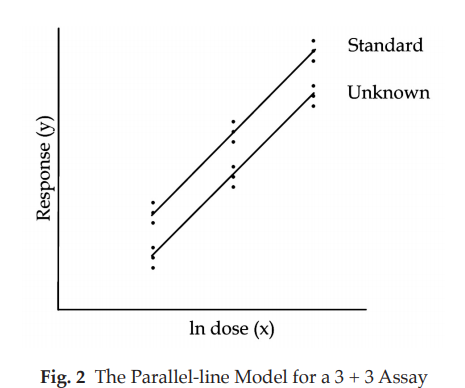
         For a drug that is assayed biologically, the response should plot as a straight line against the log-dose over an adequate range of doses. The straight line representing its relationship with the response of the assay must parallel to that for the standard.

The parallel-line model is illustrated in Fig. 2. The logarithm of the doses are represented on the horizontal axis with the lowest concentration on the left and the highest concentration on the right. The responses are indicated on the vertical axis. The individual responses to each treatment are indicated with black dots. The two lines are the calculated ln (dose)-response relationship for the standard and the unknown.

(Note The natural logarithm, ln or log_e, is used throughout this text. Wherever the term “antilogarithm”, antiln or antilog_e, is used, the quantity e^x is meant. However, the Briggs or “common” logarithm, log or log₁₀, can equally well be used. In this case the corresponding antilogarithm is 10^x .)

         For a satisfactory assay the assumed potency of the unknown must be close to the true potency. On the basis of this assumed potency and the assigned potency of the standard, equipotent dilutions (if feasible) are prepared, i.e. corresponding doses of standard and unknown are expected to give the same response. If no information on the assumed potency is available, preliminary assays are carried out over a wide range of doses to determine the range where the curve is linear.

         The more nearly correct the assumed potency of the unknown, the closer the two lines will be together, for they should give equal responses at equal doses. The horizontal distance between the lines represents the “true” potency of the unknown, relative to its assumed potency. The greater the distance between the two lines, the poorer the assumed potency of the unknown. If the line of the unknown is situated to the right of the standard, the assumed potency was overestimated, and the calculations will indicate an estimated potency lower than the assumed potency. Similarly, if the line of the unknown is situated to the left of the standard, the assumed potency was underestimated, and the calculations will indicate an estimated potency higher than the assumed potency.

         3.1.2.2 Assay design

         The following considerations will be useful in optimizing the precision of the assay design:

         ---- the ratio between the slope and the residual error should be as large as possible,

         ---- the range of doses should be as large as possible,

         ---- the lines should be as close together as possible, i.e. the assumed potency should be a good estimate of the true potency.

         The allocation of experimental units (animals, tubes, etc.) to different treatments may be made as follows:

---- completely randomized design (See Section 3.1.2.4),

---- randomized block design (See Section 3.1.2.5),

---- Latin square design (See Section 3.2.1.6), and

---- cross-over design (See Section 3.1.2.7).

3.1.2.3 Tests of validity

         Assay results are said to be “statistically valid” if the outcome of the analysis of variance is as follows.

a. The linear regression term is significant, i.e. the calculated probability is less than 0.05. If this criterion is not met, it is not possible to calculate 95 per cent confidence limits.

b. The term for non-linearity is not significant, i.e. the calculated probability is not less than 0.05. This indicates that Condition 4A, Section 3.1.1.2, is satisfied.

c. The term for non-parallelism is not significant, i.e. the calculated probability is not less than 0.05. This indicates that Condition 5A, Section 3.1.1.2, is satisfied.

         A significant deviation from parallelism in a multiple assay may be due to the inclusion in the assay design of a preparation to be examined that gives an ln (dose)-response line with a slope different from those for the other preparations. Instead of declaring the whole assay invalid, it may then be decided to eliminate all data relating to that preparation and to restart the analysis from the beginning.

         When statistical validity is established, potencies and confidence limits may be estimated by the methods described in the example under each design.

3.1.2.4 Completely randomized design

         If the totality of experimental units appears to be reasonably homogeneous with no indication that variability in response will be smaller within certain recognizable sub-groups, the allocation of the units to the different treatments should be made randomly.

         If units in sub-groups such as physical positions or experimental days are likely to be more homogeneous than the totality of the units, the precision of the assay may be increased by introducing one or more restrictions into the design. A careful distribution of the units over these restrictions permits irrelevant sources of variation to be eliminated. The statistical method of calculation is illustrated in Example 1.

Example 1 Three-Dose Single Assay, Completely Randomized Design

         The assay is composed of the standard of three concentrations, designated s1, s2 and s3 and one unknown of similar three concentrations, designated u1, u2 and u3, respectively.

          All six concentrations of standard and unknown are allocated randomly using a standard table of random numbers.

Table 1 Response y (Absorbance*)

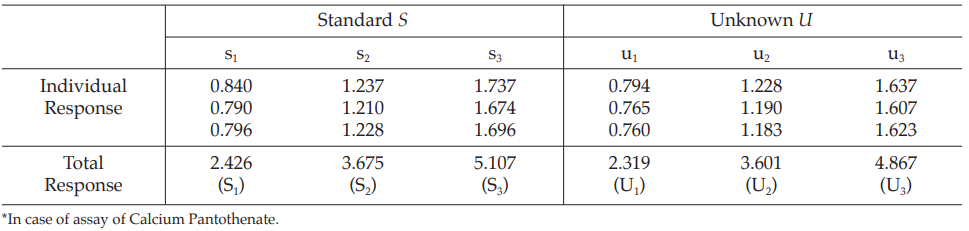
Table 2 Response Totals and Contrasts​

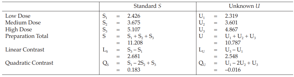
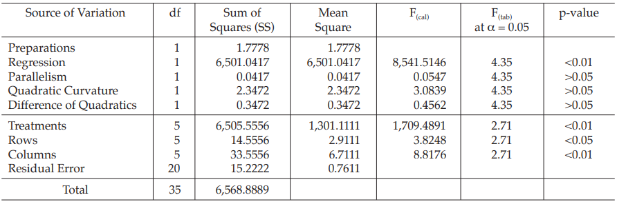
Table 3 Analysis of Variance​

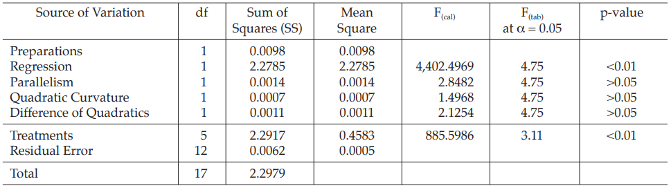
Mean Square = Sum of Squares/df

F_(cal) = Mean Square/Mean Square of Residual Error

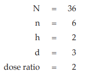
Given statistic values for the next steps:

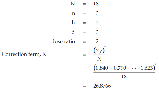
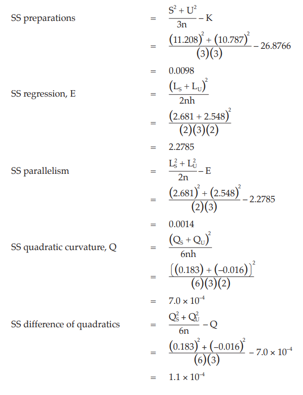
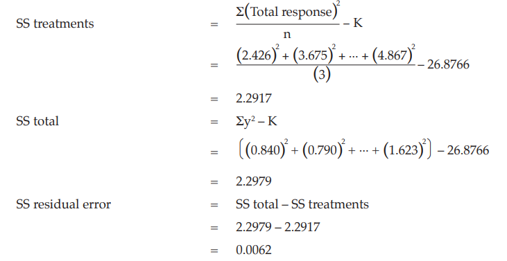
Calculation of sums of squares (SS) of the variations:

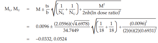
Calculation of potency ratio and confidence limits: ​

Given statistic values for the next steps:

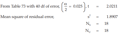
Calculate and apply ln confidence limits to the ln potency ratio: (M_L, M_U)

Confidence limits are given by antiln M_L and antiln M_L: antiln M_L = 0.8943 and anitn M_U = 0.9635.

         Thus, the potency is estimated to be 92.83 per cent of the stated potency, with confidence limits at 89.43 per cent and 96.35 per cent of the stated potency.

         If the precision of the assay is limited to be not less than 95.0 per cent and not more than 105.0 per cent of the estimated potency, the confidence limits of error will be 88.19 and 97.47 per cent of the estimated potency.

Therefore, they imply such assay precision.

3.1.2.5 Randomized block design

         In this design it is possible to segregate an identifiable source of variation, such as the sensitivity variation between litters of experimental animals or the variation between Petri dishes in a diffusion microbiological assay. The design requires that every treatment be applied an equal number of times in every block (litter or Petri dish) and is suitable only when the block is large enough to accommodate all treatments once. This is illustrated in Examples 2 to 5. It is also possible to use a randomized design with repetitions. The treatments should be allocated randomly within each block.

Example 2 Two-Dose Single Assay, Randomized Block Design

The assay is composed of one standard and two concentrations, designated s₁ and s₂ and one unknown of similar two concentrations, designated u₁ and u₂ respectively.

Table 4 Response y (Degree of Calcification*)

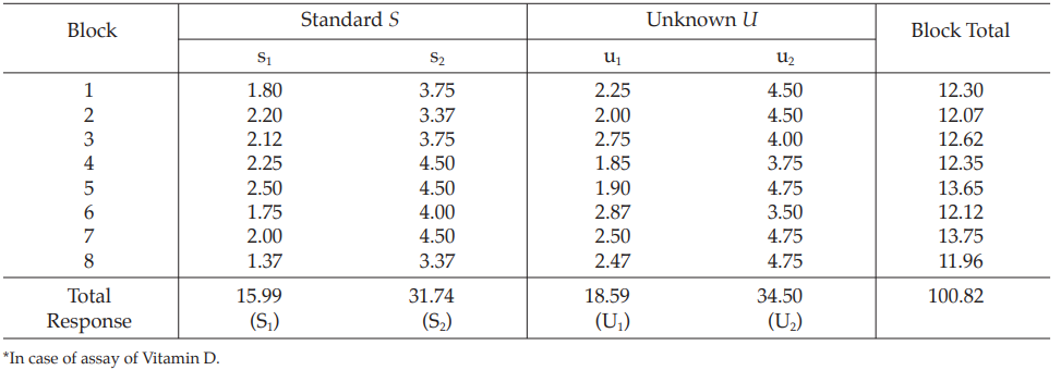
Table 5 Response Totals and Contrasts​

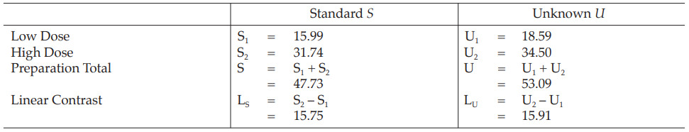
Table 6 Analysis of Variance​

Mean Square = Sum of Squares/df

F_(cal) = Mean Square/Mean Square of Residual Error

Given statistic values for the next steps:

Calculation of sums of squares (SS) of the variations:​

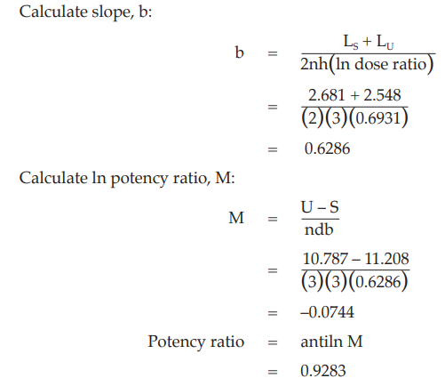
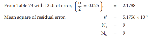
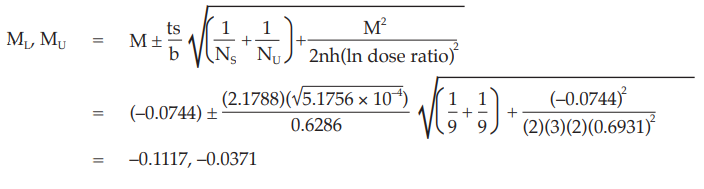
Calculation of potency ratio and confidence limits:​

Given statistic values for the next steps:​

Calculate and apply ln confidence limits to the ln potency ratio: (M_L, M_U )

Confidence limits are given by antiln M_L and antiln M_U: antiln M_L = 0.9989 and antiln M_U = 1.2660

         Thus, the potency is estimated to be 112.45 per cent of the stated potency, with confidence limits at 99.89 per cent and 126.60 per cent of the stated potency.

         If the precision of the assay is limited to be not less than 95.0 per cent and not more than 105.0 per cent of the estimated potency, the confidence limits of error will be 106.83 and 118.07 per cent of the estimated potency.

         Therefore, they do not imply such assay precision. The assay must be repeated and the combination of potency estimates is required.

Example 3 Three-Dose Single Assay, Randomized Block Design

         The assay is composed of the standard of three concentrations, designated s₁, s₂ and s₃ for 5.0, 10.0 and 20.0 μg per ml, respectively; and one unknown of similar three concentrations, designated u₁, u₂ and u₃.

         The assay requires six plates (20 mm × 100 mm), each containing six cylinders arranged in a radius pattern. In each plate, all six concentrations of standard and unknown are assigned as in Table 7. 

Table 7 A Pattern of Arrangement of Treatments

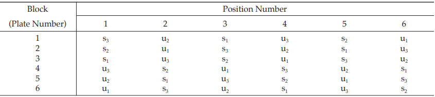
Table 8 Response y (Diameters of Inhibition Zones*, in mm × 10)

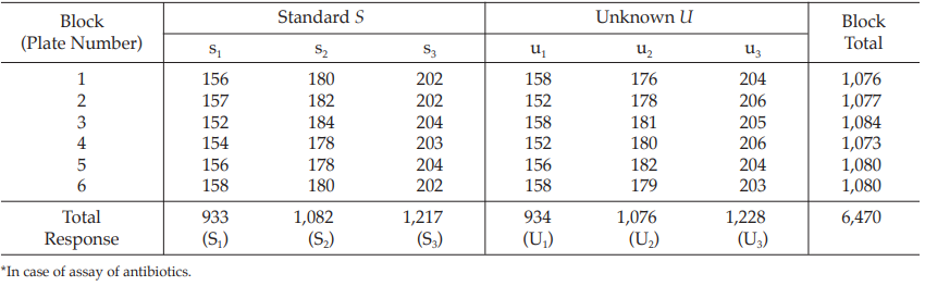
Table 9 Response Totals and Contrasts

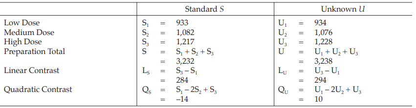
Table 10 Analysis of Variance

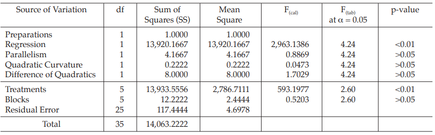
Mean Square	= Sum of Squares/df
F(cal)	= Mean Square/Mean Square of Residual Error

Given statistic values for the next steps:

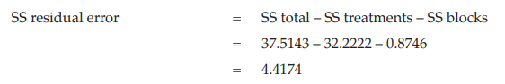
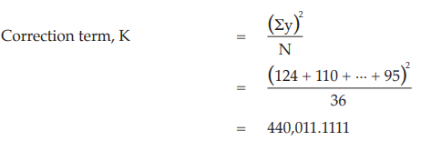
Calculation of sums of squares (SS) of the variations:​

Calculation of potency ratio and confidence limits:​

Given statistic values for the next steps:

Calculate and apply ln confidence limits to the ln potency ratio: (M_L, M_U):

Confidence limits are given by antiln M_L and antiln M_U: antiln M_L = 0.9673 and antiln M_U = 1.0538

         Thus, the potency is estimated to be 100.96 per cent of the stated potency, with confidence limits at 96.73 and 105.38 per cent of the stated potency.

          If the precision of the assay is limited to be not less than 95.0 per cent and not more than 105.0 per cent of the estimated potency, the confidence limits of error will be 95.92 and 106.01 per cent of the estimated potency.

         Therefore, they imply such assay precision.

Example 4 Three-Dose Multiple Assay, Randomized Block Design

         The assay is composed of one standard of three concentrations, designated s1, s2, and s3, and two unknowns of similar three concentrations, designated u1, u2 and u3 to z1, z2 and z3, respectively. Standard doses to be administered were 2, 4 and 8 units, and equivalent test doses are prepared assuming the potencies of the test preparations are identical to that of the standard.

         The assay required six plates (20 mm × 150 mm) each containing nine cylinders which are randomly arranged in a radius pattern as in Table 11.

Table 11 A Pattern of Arrangement of Treatments 

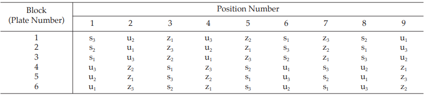
Table 12 Response y (Diameters of Inhibition Zones*, in mm × 10)​

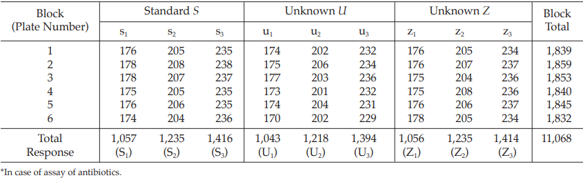
Table 13 Response Totals and Contrasts

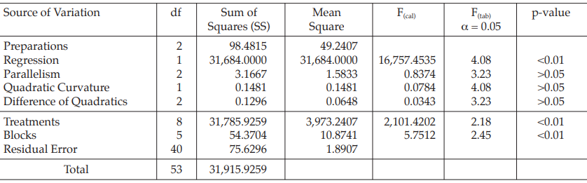
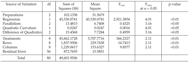
Table 14 Analysis of Variance

 

Mean Square	= Sum of Squares/df
F(cal)	= Mean Square/Mean Square of Residual Error

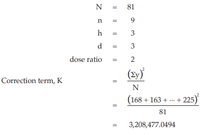
Given statistic values for the next steps:

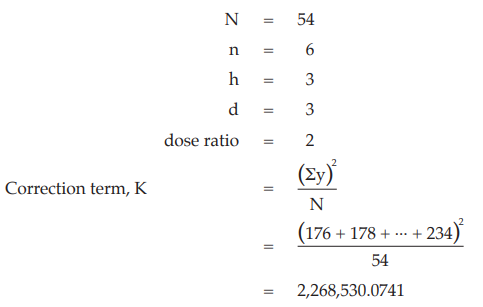
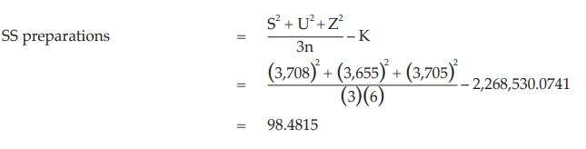
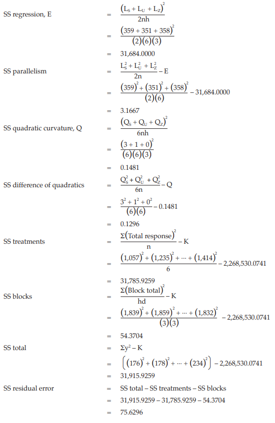
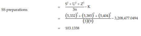
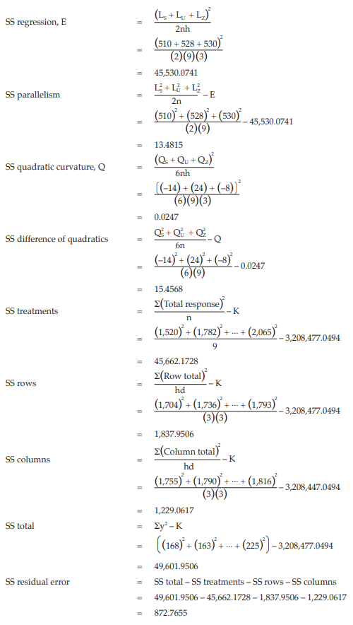
Calculation of sums of squares (SS) of the variations:​

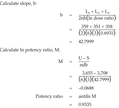
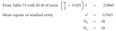
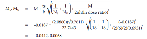
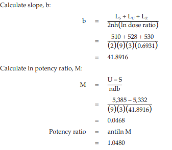
Calculation of potency ratio and confidence limits:

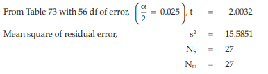
Given statistic values for the next steps:

Calculate and apply ln confidence limits to the ln potency ratio (M_L, M_U):

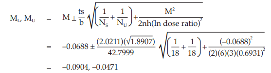
Confidence limits are given by antiln M_L and antiln M_U: antiln M_L = 0.9135 and antiln M_U = 0.9540

         Thus, the potency is estimated to be 93.35 per cent of the stated potency, with confidence limits at 91.35 and 95.40 per cent of the stated potency.

         Using the same procedure, the potency for unknown Z is 99.61 per cent of the stated potency with confidence limits at 97.48 and 101.79 per cent of the stated potency.

          If the precision of the assay is limited to be not less than 95.0 per cent and not more than 105.0 per cent of the estimated potency, the confidence limits of error of unknown U will be 88.68 and 98.02 per cent of the estimated potency, and of unknown Z will be 94.63 and 104.59 per cent of the estimated potency.

         Therefore, they imply such assay precision.

Example 5 Four-Dose Multiple Assay, Randomized Block Design

         The assay is composed of one standard of four concentrations, designated s₁, s₂, s₃ and s₄, and two or more unknowns of similar four concentrations, designated u₁, u₂, u₃ and u₄ to z₁, z₂, z₃ and z₄, respectively

Table 15 Response y (Fluorescence Intensity*)

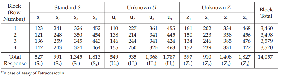
Table 16 Response Totals and Contrasts​

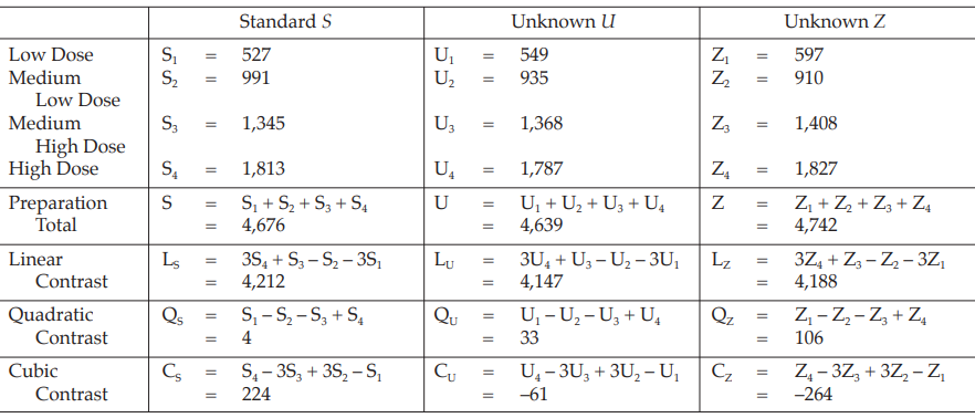
Table 17 Analysis of Variance​

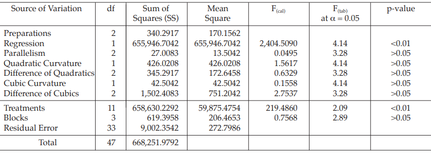
Mean Square	= Sum of Squares/df
F(cal)	= Mean Square/Mean Square of Residual Error

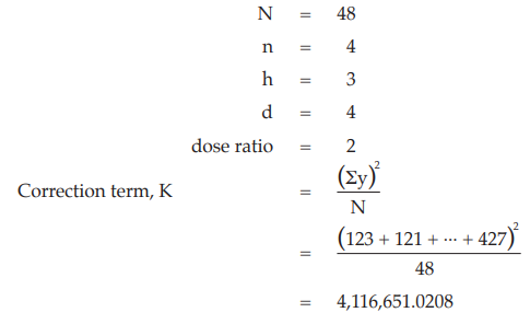
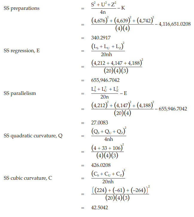
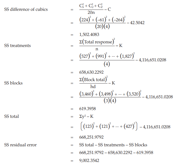
Given statistic values for the next steps:

Calculation of potency ratio and confidence limits:

Given statistic values for the next steps:

Calculate and apply ln confidence limits to the ln potency ratio (M_L, M_U):

Confidence limits are given by antiln M_L and antiln M_U: antiln M_L = 0.9102 and antiln M_U = 1.0655.

         Thus, the potency is estimated to be 98.48 per cent of the stated potency, with confidence limits at 91.02 and 106.55 per cent of the stated potency.

         Using the same procedure, the potency for unknown Z is 102.77 per cent of the stated potency with confidence limits at 94.99 and 111.20 per cent of the stated potency.

         If the precision of the assay is limited to be not less than 95.0 per cent and not more than 105.0 per cent of the estimated potency, the confidence limits of error of unknown U will be 93.55 and 103.40 per cent of the estimated potency, and of unknown Z will be 97.63 and 107.91 per cent of the estimated potency.

         Therefore, they do not imply such assay precision. The assay must be repeated and the combination of potency estimates is required.

3.1.2.6 Latin square design

         This design is appropriate when the response may be affected by two different sources of variation each of which can assume k different levels or positions. For example, in a plate assay of an antibiotic the treatments may be arranged in a k × k array on a large plate, each treatment occurring once in each row and each column. The design is suitable when the number of rows, the number of columns and the number of treatments are equal. Responses are recorded in a square format known as a Latin square. Variations due to differences in response among the k rows and among the k columns may be segregated, thus reducing the error. This design is illustrated in Examples 6 to 7.

Example 6 Three-Dose Single Assay, Latin Square Design

         The assay is composed of the standard of three concentrations, designated s₁, s₂ and s3 for 5.0, 10.0 and 20.0 μg per ml, respectively; and one unknown of similar three concentrations, designated u₁, u₂ and u₃.

         All six concentrations of the standard and the unknown are assigned to a standard square plate with a 6 × 6 pattern in such a way that each column and each row consists of all six treatments. 

Table 18 A Pattern of Arrangement of Treatments

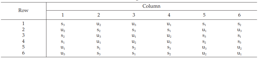
Table 19 Measured Inhibition Zones in mm × 10

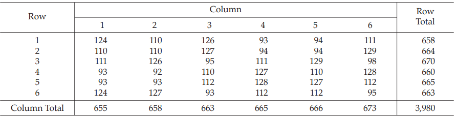
Table 20 Response y (Diameters of Inhibition Zones*, in mm × 10)

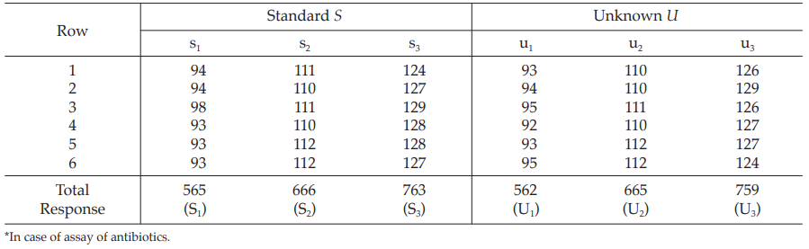
Table 21 Response Totals and Contrasts

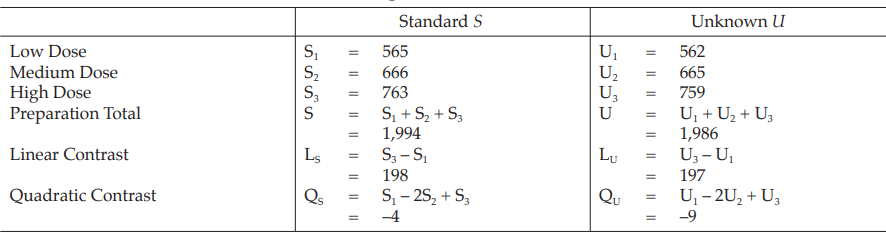
Table 22 Analysis of Variance 

Mean Square	= Sum of Squares/df
F(cal)	= Mean Square/Mean Square of Residual Error

Given statistic values for the next steps:

Calculation of sums of squares (SS) of the variations:

Calculation of potency ratio and confidence limits:​

Given statistic values for the next steps:​

Calculate and apply ln confidence limits to the ln potency ratio (M_L, M_U):

Confidence limits are given by antiln M_L and antiln M_U: antiln M_L = 0.9567 and antiln M_U = 1.0069.

Thus, the potency is estimated to be 98.15 per cent of the stated potency, with confidence limits at 95.67 and 100.69 per cent of the stated potency.

          If the precision of the assay is limited to be not less than 95.0 per cent and not more than 105.0 per cent of the estimated potency, the confidence limits of error will be 93.24 and 103.05 per cent of the estimated potency.

          Therefore, they imply such assay precision.

Example 7 Three-Dose Multiple Assay, Latin Square Design

          Standard doses to be administered were 3, 6 and 12 units, and equivalent unknown doses are prepared assuming the potencies of the unknown and the standard preparations are equal. 

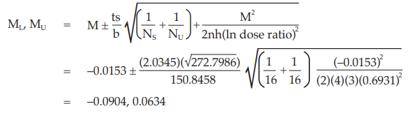
Table 23 A Pattern of Arrangement of Treatments

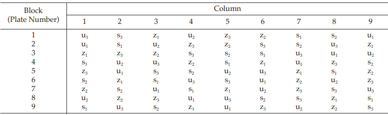
Table 24 Measured Inhibition Zones in mm × 10

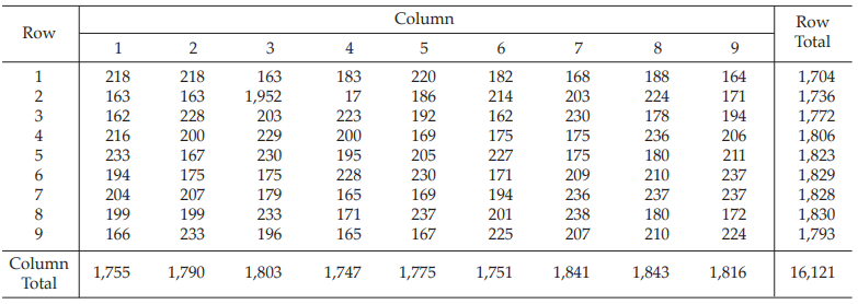
Table 25 Response y (Diameters of Inhibition Zones*, in mm × 10)

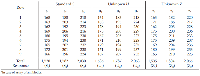
Table 26 Response Totals and Contrasts

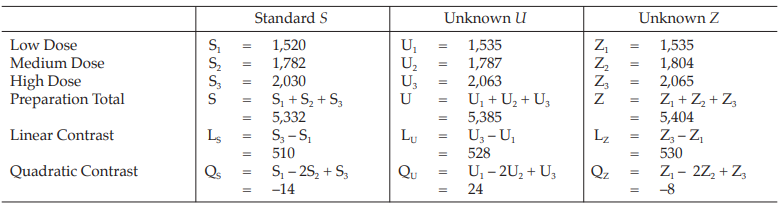
Table 27 Analysis of Variance

Mean Square	= Sum of Squares/df
F(cal)	= Mean Square/Mean Square of Residual Error

Given statistic values for the next steps:

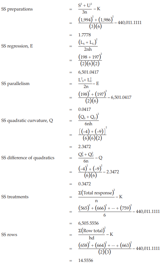
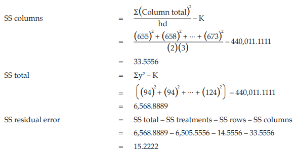
Calculation of sums of squares (SS) of the variations:​

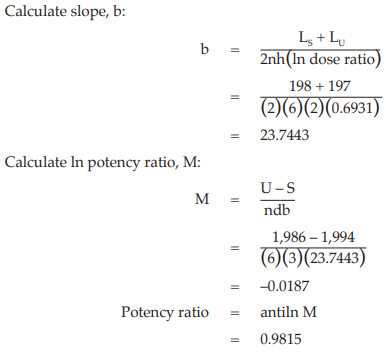
Calculation of potency ratio and confidence limits:​

Given statistic values for the next steps:​

Calculate and apply ln confidence limits to the ln potency ratio (M_L, M_U):

Confidence limits are given by antiln M_L and antiln M_U: antiln ML = 0.9955 and antiln M_U = 1.1033

          Thus, the potency is estimated to be 104.80 per cent of the stated potency, with confidence limits at 99.55 and 110.33 per cent of the stated potency.

          Using the same procedure, the potency for unknown Z is 106.57 per cent of the stated potency with confidence limits at 101.23 and 112.20 per cent of the stated potency.

          If the precision of the assay is limited to be not less than 95.0 per cent and not more than 105.0 per cent of the estimated potency, the confidence limits of error of unknown U will be 99.56 and 110.04 per cent of the estimated potency, and of unknown Z will be 101.24 and 111.90 per cent of the estimated potency.

          Therefore, they do not imply such assay precision. The assay must be repeated and the combination of potency estimates is required.

3.1.2.7 Cross-over design

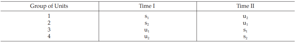
          This design is useful when the experiment can be sub-divided into blocks but it is possible to apply only two treatments to each block. For example, a block may be a single unit that can be tested on two occasions. The design is intended to increase precision by eliminating the effects of differences between units while balancing the effect of any difference between general levels of response at the two occasions. If two doses of a standard (s₁, s₂) and of an unknown (u₁, u₂) preparation are tested, this is known as a twin cross-over test.

          The experiment is divided into two parts separated by a suitable time interval. Units are divided into four groups and each group receives one of the four treatments in the first part of the test. Units that received one preparation in the first part of the test receive the other preparation on the second occasion, and units receiving small doses in one part of the test receive large doses in the other. The arrangement of doses is shown in Table 28. The statistical method of calculation is illustrated in Example 8.

Table 28 Arrangement of Doses in Cross-over Design

Example 8 Two-Dose Single Assay, Twin Cross-Over Design

The assay is composed of the standard of two concentrations, designated s₁ and s₂ and one unknown of similar two concentrations, u₁ and u₂, respectively.

Table 29 A Pattern of Arrangement of Treatments

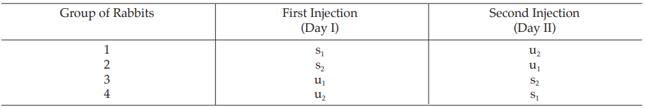
Table 30 Response y (Blood Glucose Readings, mg%)* at 1 (y1) and 2 (y2) Hours

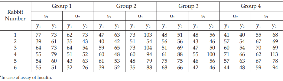
Table 31 Response y (Sum of Blood Glucose Concentrations, mg%, at 1 and 2 Hours)

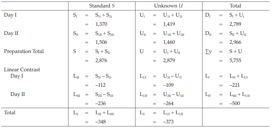
Table 32 Response Totals and Contrasts

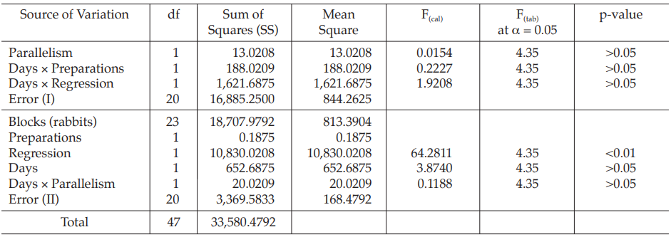
Table 33 Analysis of Variance

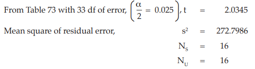
Given statistic values for the next steps:

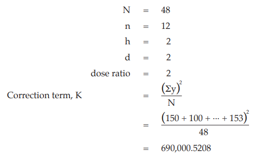
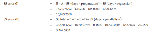
Calculation of sums of squares (SS) of the variations:​

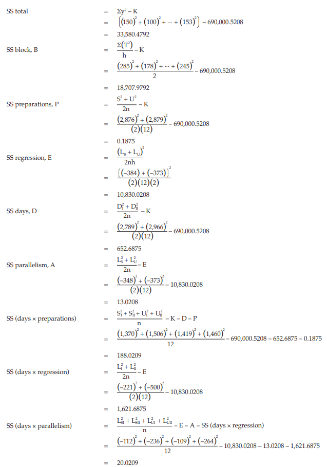
Calculation of potency ratio and confidence limits:​

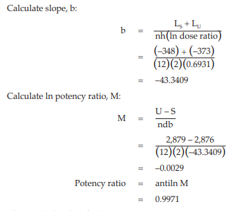
Given statistic values for the next steps:​

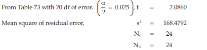
Calculate and apply ln confidence limits to the ln potency ratio (M_L, M_U):

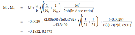
Confidence limits are given by antiln M_L and antiln M_U: antiln M_L = 0.8326 and antiln M_U = 1.1942.

          Thus, the potency is estimated to be 99.71 per cent of the stated potency, with confidence limits at 83.26 and 119.42 per cent of the stated potency.

           If the precision of the assay is limited to be not less than 95.0 per cent and not more than 105.0 per cent of the estimated potency, the confidence limits of error will be 94.73 and 104.70 per cent of the estimated potency.

          Therefore, they do not imply such assay precision. The assay must be repeated and the combination of potency estimates is required.

3.1.2.8 Missing values

          In a balanced assay, an accident totally unconnected with the applied treatments may lead to the loss of one or more responses, for example, because an animal dies. If it is considered that the accident is in no way connected with the composition of the preparation administered, the exact calculations can still be performed but the formulae are necessarily more complicated and can only be given within the framework of general linear models. However, there exists an approximate method which keeps the simplicity of the balanced design by replacing the missing response by a calculated value. The loss of information is taken into account by diminishing the degrees of freedom for the total sum of squares and for the residual error by the number of missing values and using one of the formulae below for the missing values. It should be borne in mind that this is only an approximate method, and that the exact method is to be preferred.

          If more than one observation is missing, the same formulae can be used. The procedure is to make a rough guess at all the missing values except one, and to use the proper formula for this one, using all the remaining values including the rough guesses. Fill in the calculated value. Continue by similarly calculating a value for the first rough guess. After calculating all the missing values in this way the whole cycle is repeated from the beginning, each calculation using the most recent guessed or calculated value for every response to which the formula is being applied. This continues until two consecutive cycles give the same values; convergence is usually rapid.

          Provided that the number of values replaced is small relative to the total number of observations in the full experiment (say less than 5 per cent), the approximation implied in this replacement and reduction of degrees of freedom by the number of missing values so replaced is usually fairly satisfactory. The analysis should be interpreted with great care, however, especially if there is a preponderance of missing values in one treatment or block, and a biometrician should be consulted if any unusual features are encountered. Replacing missing values in a test without replication is a particularly delicate operation.

Completely randomized design

          In a completely randomized assay the missing value can be replaced by the arithmetic mean of the other responses to the same treatment.

Randomized block design

The missing value (y’) is obtained by the use of:

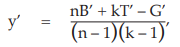
where B’ and T’ are the sum of the remaining responses in the block and treatment, respectively, containing the missing value, G’ is the sum of all remaining responses recorded in the assay, and n and k are the number of blocks and treatments, respectively.

          As an example, suppose that the response to dose s1 in the first block of the results obtained from Example 3 was missing:

Calculate the missing value 

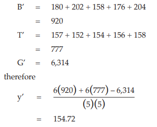
          The value 154.72 would appear in Table 8 in place of 156 and calculation would proceed as in Example 3, but the degrees of freedom for the residual error and for total sum of squares would be 24 and 34, respectively.

Latin square design

The missing value (y’) is obtained by the use of:

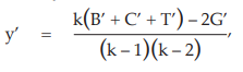
where B’, C’ and T’ are the sums of the remaining responses in the row, column and treatment, respectively, containing the missing value. In this case, number of rows, columns and treatments are equal.

          As an example, suppose that the response in the first row and first column (s₃) of the results obtained from Example 6 was missing:

Calculate the missing value

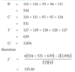
          The value 125.6 would appear in Tables 19 and 20 in place of 124 and calculation would proceed as in Example 6, but the degrees of freedom for the residual error and for the total sum of squares would be 19 and 34, respectively.

Cross-over design

                    If an accident leading to loss of values occurs in a cross-over design, a book on statistics should be consulted, because the appropriate formulae depend upon the particular treatment combinations.

3.1.3 The slope-ratio model

3.1.3.1 Introduction

          This model is suitable, for example, for some microbiological assays when the independent variable is the concentration of an essential growth factor below the optimal concentration of the medium. The slope-ratio model is illustrated in Fig. 3.

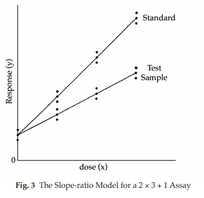
          The doses are represented on the horizontal axis with zero concentration on the left and the highest concentration on the right. The responses are indicated on the vertical axis. The individual responses to each treatment are indicated with black dots. The two lines are the calculated dose-response relationship for the standard and the unknown under the assumption that they intersect each other at zero-dose. Unlike the parallel-line model, the doses are not transformed to logarithms.

          Just as in the case of an assay based on the parallel-line model, it is important that the assumed potency is close to the true potency, and to prepare equipotent dilutions of the test preparations and the standard (if feasible). The more nearly correct the assumed potency, the closer the two lines will be together. The ratio of the slopes represents the “true” potency of the unknown, relative to its assumed potency. If the slope of the unknown preparation is steeper than that of the standard, the potency was underestimated and the calculations will indicate an estimated potency higher than the assumed potency. Similarly, if the slope of the unknown is less steep than that of the standard, the potency was overestimated and the calculations will result in an estimated potency lower than the assumed potency.

          In setting up an experiment, all responses should be examined for the fulfillment of conditions 1, 2 and 3 in Section 3.1.1.

3.1.3.2 Assay design

          The use of the statistical analysis presented below imposes the following restrictions on the assay:

a. the standard and the test preparations must be tested with the same number of equally spaced dilutions,

b. an extra group of experimental units receiving no treatment may be tested (the blanks),

c. there must be an equal number of experimental units to each treatment.

          As already remarked in Section 3.1.1.3, assay designs not meeting these restrictions may be both possible and correct, but the simple statistical analyses presented here are no longer applicable and either expert advice should be sought or suitable software should be used.

          A design with two doses per preparation and one blank, the “common zero (2h + 1)-design”, is usually preferred, since it gives the highest precision combined with the possibility to check validity within the constraints mentioned above. However, a linear relationship cannot always be assumed to be valid down to zero-dose. With a slight loss of precision a design without blanks may be adopted. In this case three doses per preparation, the “common zero (3h)-design”, are preferred to two doses per preparation. The doses are thus given as follows:

1) the standard is given in a high dose, near to but not exceeding the highest dose giving a mean response on the straight portion of the dose-response line,

2) the other doses are uniformly spaced between the highest dose and zero-dose,

3) the test preparations are given in corresponding doses based on the assumed potency of the material.

          A completely randomized, a randomized block or a latin square design may be used, such as described in Section 3.1.2.4 to 3.1.2.6. The use of any of these designs necessitates an adjustment to the error sum of squares as described in Examples 1 to 6. The analysis of an assay of one or more test preparations against a standard is described below.

3.1.3.3 Tests of validity

          Assay results are said to be “statistically valid” if the outcome of the analysis of variance is as follows:

          a) the variation due to blanks in (hd + 1)-designs is not significant, i.e. the calculated probability is not smaller than 0.05. This indicates that the responses of the blanks do not significantly differ from the common intercept and the linear relationship is valid down to zero-dose;

          b) the variation due to intersection is not significant, i.e. the calculated probability is not less than 0.05. This indicates that condition 5B, Section 3.1.1 is satisfied;

          c) in assays including at least three doses per preparation, the variation due to non-linearity is not significant, i.e. the calculated probability is not less than 0.05. This indicates that condition 4B, Section 3.1.1 is satisfied.

          A significant variation due to blanks indicates that the hypothesis of linearity is not valid near zero-dose. If this is likely to be systematic rather than incidental for the type of assay, the (hd)-design is more appropriate. Any response to blanks should then be disregarded.

          When statistical validity is established, potencies and confidence limits may be estimated by the methods described in the Examples 9 and 10.

3.1.3.4 Completely randomized design

          In this design, it is recommended to test the validity of assay results as described in Section 3.1.3.3. The (hd + 1)-design is applicable, if conditions a), b), and c) are satisfied (See Example 9). If only conditions b) and c) are satisfied (See Example 10), the (hd)-design is more appropriate.

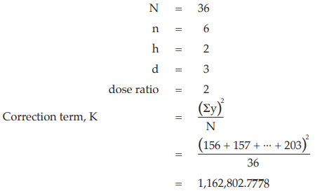
Example 9 Slope-ratio Assay, Completely Randomized (0,3,3)-design

          The assay is composed of the standard of three dilutions, designated s₁, s₂ and s₃ and one unknown of similar three dilutions, designated u₁, u₂ and u₃, respectively. In addition a blank is prepared, although a linear doseresponse relationship is not expected for low doses.

          Eight replications of each dilution are prepared.

Table 34 Response y (Absorbance*)

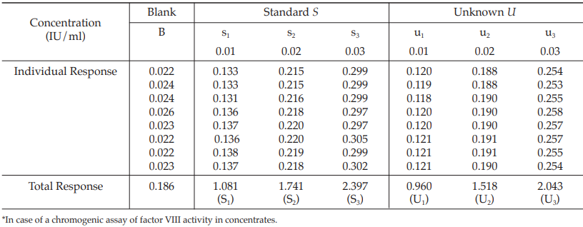
Table 35 Response Totals and Contrasts

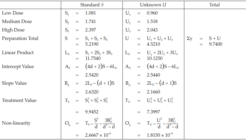
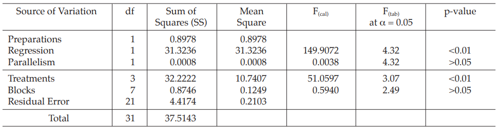
Table 36 Analysis of Variance

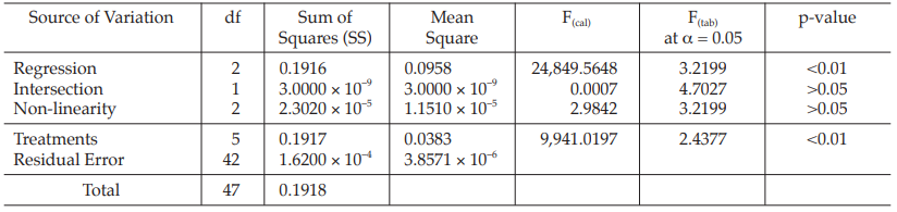
Mean Square	= Sum of Squares/df
F(cal)	= Mean Square/Mean Square of Residual Error

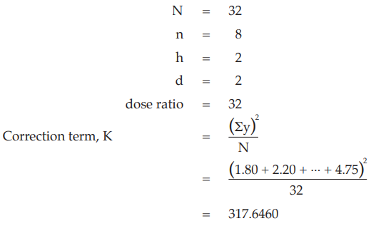
Given statistic values for the next steps:

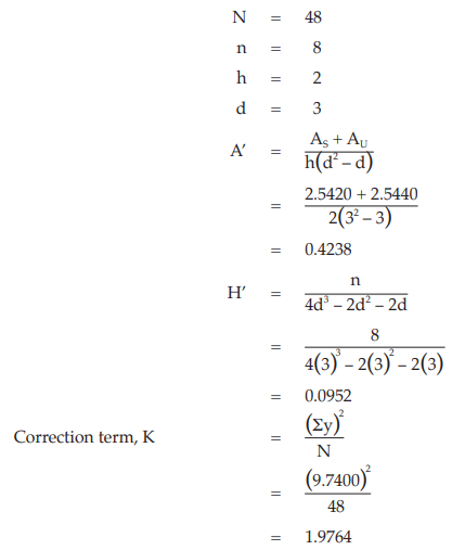
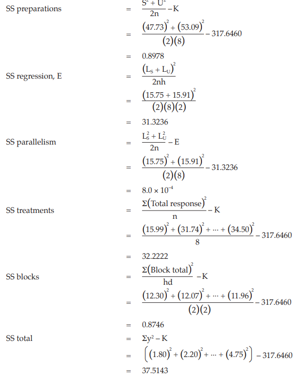
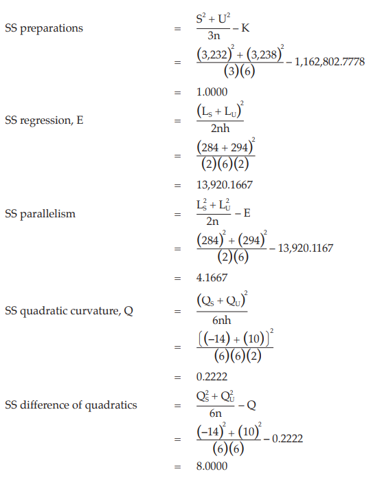
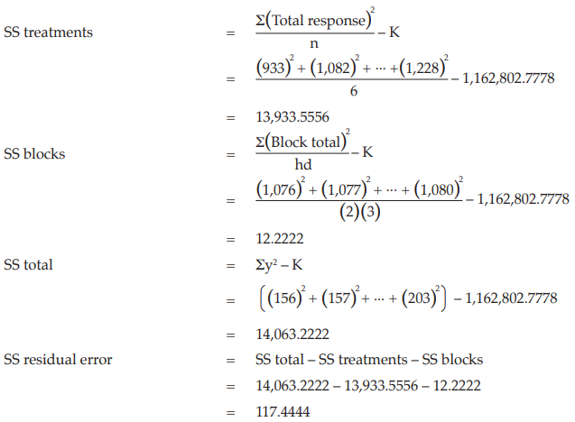
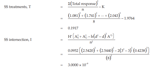
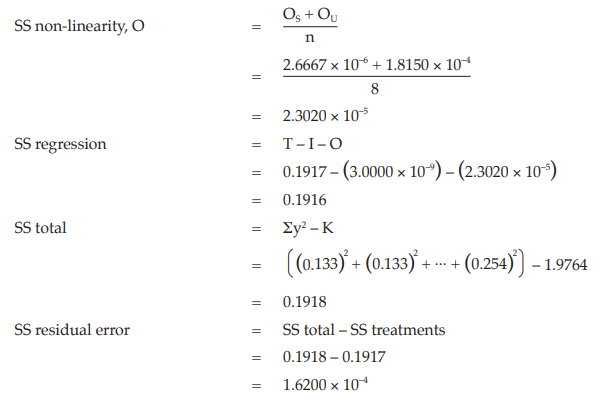
Calculation of sums of squares (SS) of the variations:​

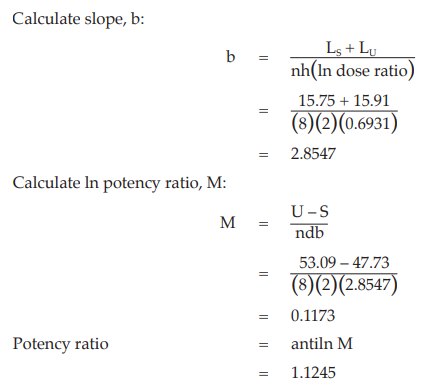
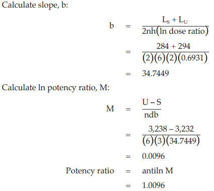
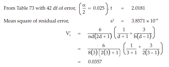
Calculation of potency ratio and confidence limits:​

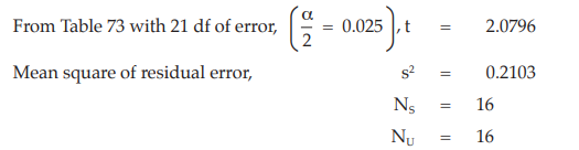
Given statistic values for the next steps:

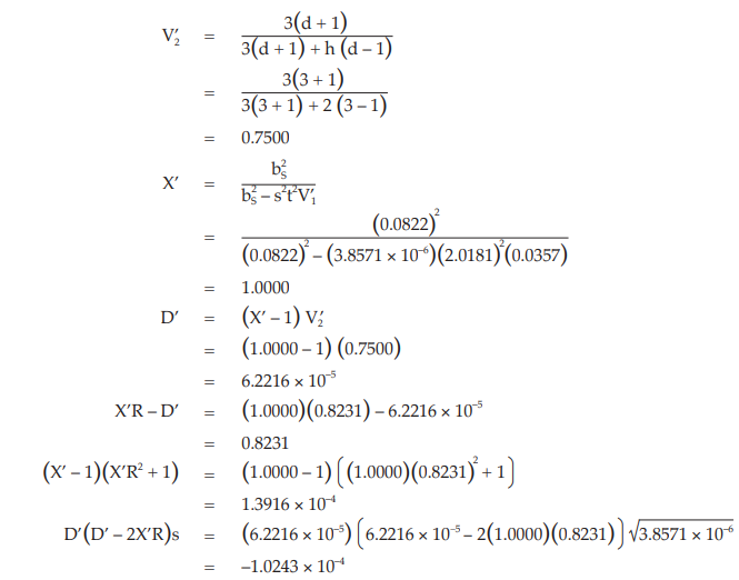
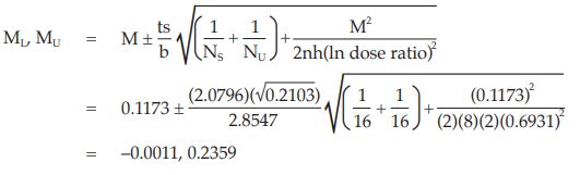
Calculate and apply ln confidence limits to the potency ratio (lower limit, upper limit):

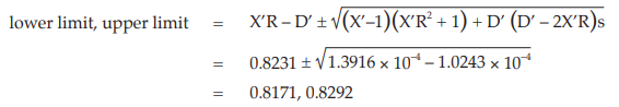
          Thus, the potency is estimated to be 82.31 per cent of the stated potency, with confidence limits at 81.71 and 82.92 per cent of the stated potency.

          If the precision of the assay is limited to be not less than 95.0 per cent and not more than 105.0 per cent of the estimated potency, the confidence limits of error will be 78.19 and 86.43 per cent of the estimated potency.

          Therefore, they imply such assay precision.

Example 10 Slope-ratio Assay, Completely Randomized (0,4,4,4)-design

          The assay is composed of the standard of four dilutions, designated s₁, s₂, s₃ and s₄ and two or more unknowns of similar four dilutions, designated u₁, u₂, u₃ and u₄ to z₁, z₂, z₃ and z₄, respectively.

          Two replications of each dilution are prepared.

Table 37 Response y (Absorbance*)

Table 38 Response Total and Contrasts

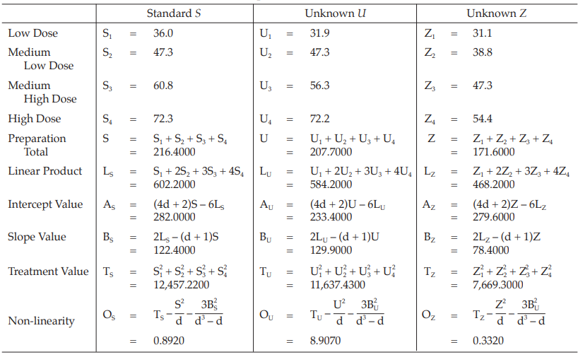
Table 39 Analysis of Variance

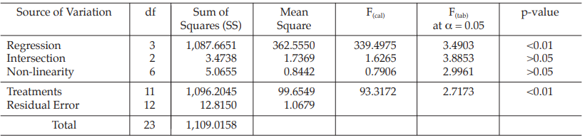
Mean Square	= Sum of Squares/df
F(cal)	= Mean Square/Mean Square of Residual Error

Given statistic value for the next steps:

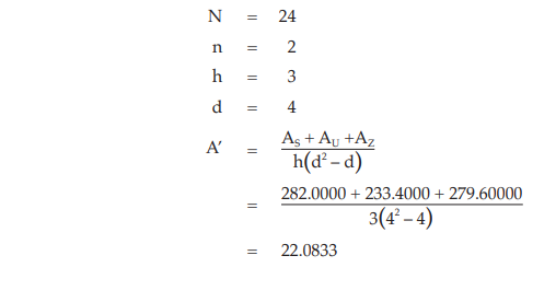
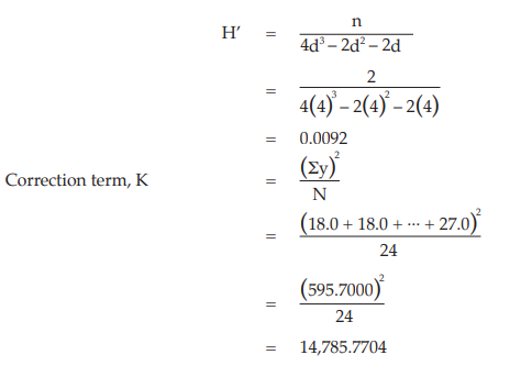
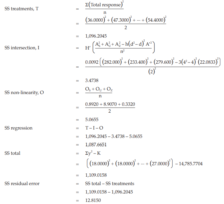
Calculation of sums of squares (SS) of the variations:

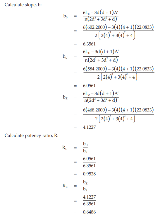
Calculation of potency ratio and confidence limits:

Given statistic values for the next steps:

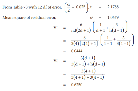
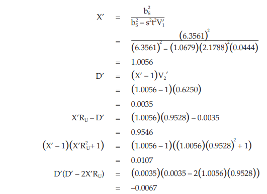
Calculate and apply confidence limits to the potency ratio (lower limit, upper limit):

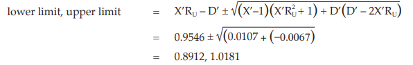
          Thus, the potency is estimated to be 95.28 per cent of the stated potency, with confidence limits at 89.12 and 101.81 per cent of the stated potency.

          Using the same procedure, the potency for unknown Z is 64.86 per cent with confidence limits at 59.03 and 70.73 per cent of the stated potency.

          If the precision of the assay is limited to be not less than 95.0 per cent and not more than 105.0 per cent of the estimated potency, the confidence limits of error of unknown U will be 90.52 and 100.04 per cent of the estimated potency, and of unknown Z will be 61.62 and 68.11 per cent of the estimated potency.

          Therefore, they do not imply such assay precision. The assay must be repeated and the combination of potency estimates is required.

3.1.4 Extended sigmoid dose-response curves

          The model is suitable, for example, for some immunoassays when analysis is required of extended sigmoid dose-response curves. This model is illustrated in Fig. 4.

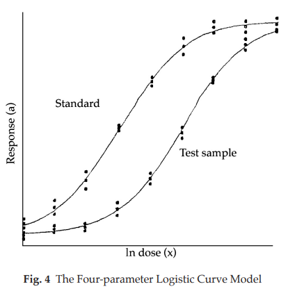
          The logarithms of the doses are represented on the horizontal axis with the lowest concentration on the left and the highest concentration on the right. The responses are indicated on the vertical axis. The individual responses to each treatment are indicated with black dots. The two curves are the calculated ln (dose)-response relationship for the standard and the test preparation.

          The general shape of the curves, an S-shaped curve can usually be described by a logistic function but other shapes are also possible. Each curve can be characterized by 4 parameters: the upper asymptote (α’), the lower asymptote (δ), the slope-factor (β), and the horizontal location (γ). This model is therefore often referred to as a fourparameter model. A mathematical representation of the ln (dose)-response curve is:

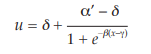
For a valid assay it is necessary that the curves of the standard and the test preparations have the same slope-factor, and the same maximum and minimum response level at the extreme parts. Only the horizontal location (γ) of the curves may be different. The horizontal distance between the curves is related to the “true” potency of the unknown. If the assay is used routinely, it may be sufficient to test the condition of equal upper and lower response levels when the assay is developed, and then to retest this condition directly only at suitable intervals or when there are changes in materials or assay conditions.

          The maximum-likelihood estimates of the parameters and their confidence intervals can be obtained with suitable computer programs. These computer programs may include some statistical tests reflecting validity. For example, if the maximum likelihood estimation shows significant deviations from the fitted model under the assumed conditions of equal upper and lower asymptotes and slopes, then one or all of these conditions may not be satisfied.

          The logistic model raises a number of statistical problems which may require different solutions for different types of assays, and no simple summary is possible. A wide variety of possible approaches is described in the relevant literature. Professional advice is therefore recommended for this type of analysis. If professional advice or suitable software is not available, alternative approaches are possible: 1) if “reasonable” estimates of the upper limit (α’) and lower limit (δ) are available, select for all preparations the doses with mean of the responses (u) falling between approximately 20 per cent and 80 per cent of the limits, transform responses of the selected doses to and use the parallel line model (Section 3.1.2) for the analysis; 2) select a range of doses for which the responses (u) orsuitably transformed responses, the selected doses to y = ln and use the parallel line model (Section 3.1.2) α’– u for the analysis; 3) select a range of doses for which the responses, for example ln (u), are approximately linear when plotted against ln (dose); the parallel line model (Section 3.1.2) may then be used for analysis.

3.2 ASSAYS DEPENDING UPON QUANTAL RESPONSES 

3.2.1 Introduction 

          In certain assays it is impossible or excessively laborious to measure the effect on each experimental unit on a quantitative scale. Instead, an effect such as death or hypoglycemic symptoms may be observed as either occurring or not occurring in each unit, and the result depends on the number of units in which it occurs. Such assays are called quantal or all-or-none.

          The situation is very similar to that described for quantitative assays in Section 3.1.1, but in place of n separate responses to each treatment a single value is recorded, i.e. the fraction of units in each treatment group showing a response. When these fractions are plotted against the logarithms of the doses the resulting curve will tend to be sigmoid (S-shaped) rather than linear. A mathematical function that represents this sigmoid curvature is used to estimate the dose-response curve. The most commonly used function is the cumulative normal distribution function. This function has some theoretical merit, and is perhaps the best choice if the response is a reflection of the tolerance of the units. If the response is more likely to depend upon a process of growth, the logistic distribution model is preferred, although the difference in outcome between the two models is usually very small. The maximum likelihood estimators of the slope and location of the curves can be found only by applying an iterative procedure. There are many procedures which lead to the same outcome, but they differ in efficiency due to the speed of convergence. One of the most rapid methods is direct optimization of the maximum-likelihood function (see Section 5.1), which can easily be performed with computer programs having a built-in procedure for this purpose. The technique described below is not the most rapid, but has been chosen for its simplicity compared to the alternatives. It can be used for assays in which one or more test preparations are compared to a standard. Furthermore, the following conditions must be fulfilled:

1) the relationship between the logarithm of the dose and the response can be represented by a cumulative normal distribution curve,

2) the curves for the standard and the test preparation are parallel, i.e. they are identically shaped and may only differ in their horizontal location,

3) in theory, there is no natural response to extremely low doses and no natural non-response to extremely high doses.

3.2.2 The probit method

          The sigmoid curve can be made linear by replacing each response, i.e. the fraction of positive responses per group, by the corresponding value of the cumulative standard normal distribution. This value, often referred to as “normit”, ranges theoretically from –∞ to +∞. In the past it was proposed to add 5 to each normit to obtain “probits”. This facilitated the hand-performed calculations because negative values were avoided. With the arrival of computers the need to add 5 to the normits has disappeared. The term “normit method” would therefore be better for the method described below. However, since the term “probit analysis” is so widely spread, the term will, for historical reasons, be maintained in this text. Probit analysis requires the iteration process to get the expected probits Y by the fitting of linear regression. All Y are set at zeros for the first iteration. The cycle is repeated until the difference between two cycles has become small (e.g., the maximum difference of Y between two consecutive cycles is smaller than 10^–8).

          Once the responses have been linearized, it should be possible to apply the parallel-line analysis as described in Section 3.1.2. Unfortunately, the validity condition of homogeneity of variance for each dose is not fulfilled. The variance is minimal at normit = 0 and increases for positive and negative values of the normit. It is therefore necessary to give more weight to responses in the middle part of the curve, and less weight to the more extreme parts of the curve. This method is illustrated in Example 11.

Example 11 Probit Analysis, An In-vivo Assay of a Diphtheria Vaccine 

        A diphtheria vaccine (assumed potency 140 IU/vial) is assayed against a standard (assigned potency 132 IU/vial). On the basis of this information, equivalent doses are prepared and randomly administered to groups of guinea-pigs. After a given period, the animals are challenged with diphtheria toxin and the number of surviving animals recorded as shown in Table 40.

         From Tables 41 to 48, the results are computerized and displayed as four decimal digits, without rounding off, except column (7).

Table 40 Raw Data from a Diphtheria Assay in Guinea-pigs

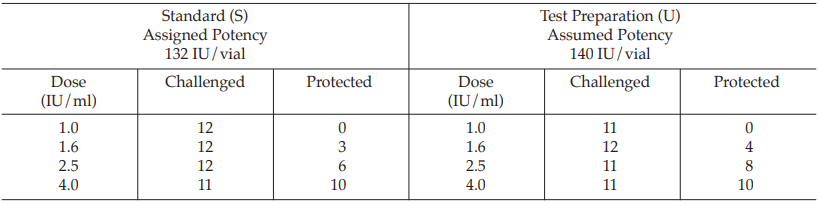
Table 41 First Working Table in the First Cycle

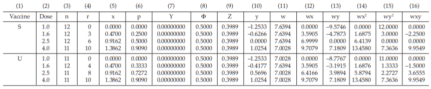
Table 42 Second Working Table in the First Cycle 

The data entered into the columns in the tables indicated by number:

(1) the vaccine label: S for standard, U for test preparation,

(2) the dose of the standard or the test preparations,

(3) the number n of replicates for each treatment,

(4) the number of positive responding units r per treatment group,

(5) the natural logarithm of the dose, x,

(6) the fraction of positive responses per group, p = 

(6) the fraction of positive responses per group, p = 

= 0.2500

For the first cycle:

(7) column Y is filled with zeros,

(8) the cumulative standard normal distribution function, Φ = Φ (Y),

for Vaccine S dose 1.6,                                        Φ = 0.5000

(9) the compute of Z,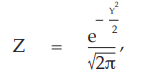                                        

for Vaccine S dose 1.6                                        

                                                                        = 0.3989

(10) the compute of y,                                      

for Vaccine S dose 1.6,                                      

                                                                        = –0.6266

(11) the compute of w,                                      

for Vaccine S dose 1.6,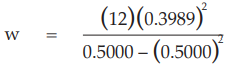                                      

                                                                         = 7.6394

The columns (12) to (16) in the first working table can be calculated from columns (5), (10) and (11) as wx, wy, wx² , wy² and wxy, respectively.

The sums calculated from columns (11) to (16) are transferred to columns (18) to (23) respectively

(24) the compute of S_xx,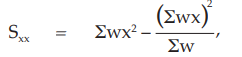                                      

for Vaccine S,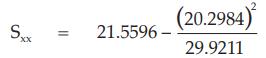                                                        

                                                                                        = 7.7892

(25) the compute of S_xy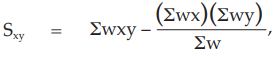                                              

for Vaccine S,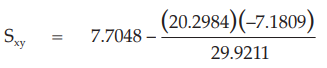                                                     

                                                                                     = 12.5764

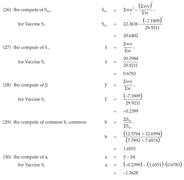
Table 43 First Working Table in the Second Cycle

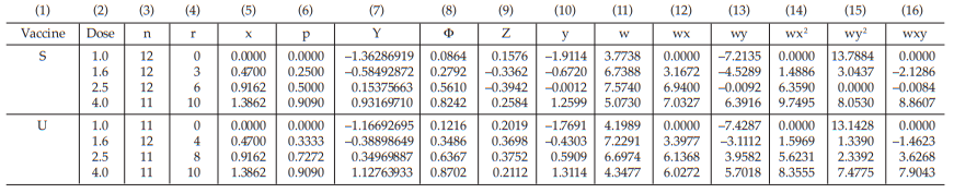
Table 44 Second Working Table in the First Cycle 

For the second cycle:

the column (7) of the first working table in the second cycle (Table 43) can be replaced by Y = a + bx (using a and b from the first cycle),

for Vaccine S dose 1.6, Y = –1.3628 + (1.6551) (0.4700) = –0.5849

The next cycles are not shown but they are repeated until the difference in Y between two consecutive cycles has become smaller than 10–8.

Tables 45 and 46 show the cycle before sufficient and Tables 47 and 48 show the sufficient cycle.

The cycles shown in Tables 47 and 48 are sufficient for the estimation.

Table 45 First Working Table in the Second Cycle 

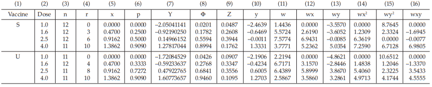
Table 46 Second Working Table in the Cycle before Sufficient

Table 47 First Working Table in the Sufficient Cycle

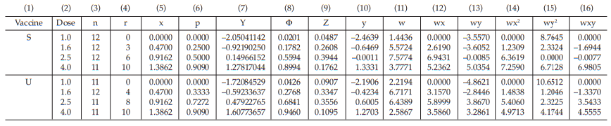
Table 48 Second Working Table in the Sufficient Cycle

Test of validity

          Before calculating the potencies and confidence interval, test for linearity and parallelism of the assay must be assessed.

Test for linearity

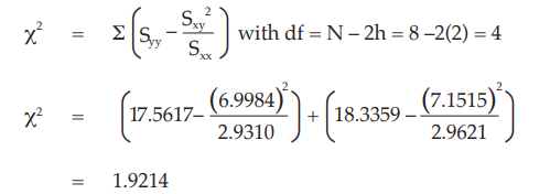
The X² with 4 degrees of freedom is 1.9214 representing a p-value of 0.7501 which is not significant deviations from linearity.

Test for parallelism:

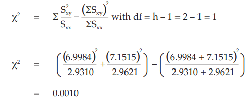
The X² with 1 degree of freedom is 0.0010 representing a p-value of 0.9742 which is not significant.

Estimation of potency and confidence limits

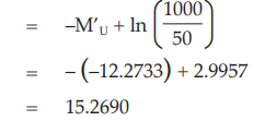
When there are no indications for a significant departure from linearity and parallelism the ln (potency ratio), M’_U, is calculated as:

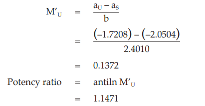
Given statistic values for the next steps:

                   

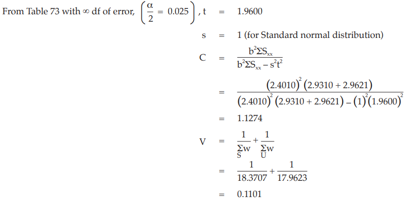
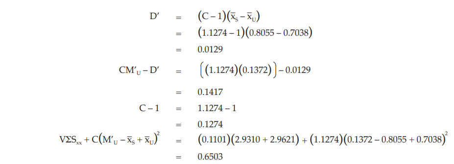
Calculate and apply ln confidence limits to ln potency ratio (M_L, M_U):

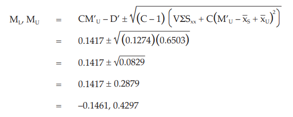
Confidence limits are given by antiln M_L and M_U: antiln M_L = 0.8640 and antiln M_U = 1.5368

          Thus, the potency is estimated to be 160.59 IU/vial with 95 per cent confidence limits from 120.97 IU/vial to 215.15 IU/vial.

          If the precision of the assay is limited to be not less than 95.0 per cent and not more than 105.0 per cent of the estimated potency, the confidence limits of error will be 152.56 IU/vial and 168.62 IU/vial of the estimated potency.

Therefore, they do not imply such assay precision. The assay must be repeated and the combination of potency estimates is required.

3.2.3 The logit method

          As indicated in Section 3.2.1 the logit method may sometimes be more appropriate. The range of these values varies from –∞ to +∞ which correspond to the cumulative standard normal distribution. The name of the method is derived from the logit function which is the inverse of the logistic distribution. The procedure is similar to that described for the probit method with the modifications as shown in Example 12.

Example 12 Logit Analysis, An In-vivo Assay of a Diphtheria Vaccine

          A diphtheria vaccine (assumed potency 140 IU/vial) is assayed against a standard (assigned potency 132/IU/ vial). On the basis of this information, equivalent doses are prepared and randomly administered to groups of guinea-pigs. After a given period, the animals are challenged with diphtheria toxin and the number of surviving animals recorded as shown in Table 49.

          From Tables 50 to 57, the results are computerized and displayed as four decimal digits, without rounding off, except column (7).

Table 49 Raw Data from a Diphtheria Assay in Guinea-pigs

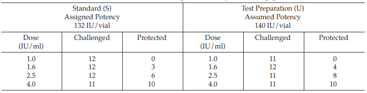
Table 50 First Working Table in the First Cycle

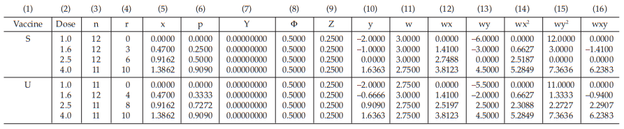
Table 51 Second Working Table in the First Cycle

The data entered into the columns in the tables indicated by number:

(1) the vaccine label: S for standard, U for test preparation,

(2) the dose of the standard or the test preparations,

(3) the number n of replicates for each treatment,

(4) the number of positive responding units r per treatment group,

(5) the natural logarithm of the dose, x,

(6) the fraction of positive responses per group, p =  

for Vaccine S dose 1.6,                          p =  

  = 0.25

For the first cycle:

(7) column Y is filled with zeros,

(8) the cumulative standard normal distribution function, 

for Vaccine S dose 1.6                         Φ = 0.5000 

(9) the compute of Z,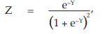                                 

for Vaccine S dose 1.6,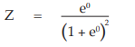                       

= 0.2500

(10) the compute of y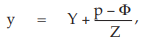                                 

for Vaccine S dose 1.6                        

= −1.0000

(11) the compute of w                                  

for Vaccine S dose 1.6,                        

= 3.0000

          The columns (12) to (16) in the first working table can be calculated from columns (5), (10) and (11) as wx, wy, wx² , wy² and wxy, respectively.

The sums calculated from columns (11) to (16) are transferred to columns (18) to (23) respectively.

(24) the compute of S_xx,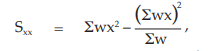                              

for Vaccine S,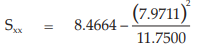                                       

= 3.0588

(25) the compute of S_xy,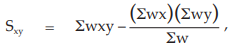                                   

for Vaccine S,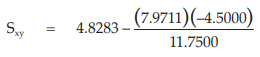                                          

    = 7.8811

(26) the compute of S_yy,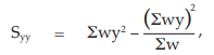                                     

for Vaccine S,                                           

     = 20.6402

(29) the compute of common b,                                

        = 2.6412 

(30) the compute of a,                                             

for Vaccine S,                                                 a = (–0.3829) – (2.6412)(0.6783)

  = –2.1748

Table 52 First Working Table in the Second Cycle

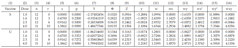
Table 53 Second Working Table in the Second Cycle

For the second cycle:

the column (7) of the first working table in the second cycle (Table 52) can be replaced by Y = a + bx (using a and b from the first cycle),

for Vaccine S dose 1.6, Y = –2.1748 + (2.6412) (0.4700) = –0.93341119

The next cycles are not shown but they are repeated until the difference in Y between two consecutive cycles has become smaller than 10–8.

Tables 54 and 55 show the cycle before sufficient and Tables 56 and 57 show the sufficient cycle.

The cycles shown in Tables 56 and 57 are sufficient for the estimation.

Table 54 First Working Table in the Cycle before Sufficient

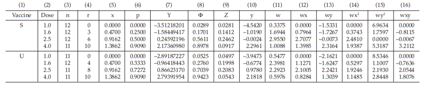
Table 55 Second Working Table in the Cycle before Sufficient

Table 56 First Working Table in the Sufficient Cycle

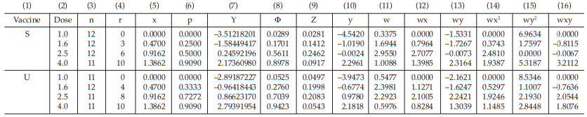
Table 57 Second Working Table in the Sufficient Cycle

Test of validity

          Before calculating the potencies and confidence interval, test for linearity and parallelism of the assay must be assessed.

Test for linearity:

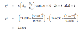
The χ² with 4 degrees of freedom is 2.1504 representing a p-value of 0.7081 which is not significant deviations from linearity.

Test for parallelism:

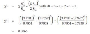
The χ² with 1 degree of freedom is 0.0066 representing a p-value of 0.9351 which is not significant.

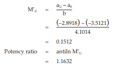
Estimation of potency and confidence limits

When there are no indications for a significant departure from linearity and parallelism the ln (potency ratio), M’_U, is calculated as:

Given statistic values for the next steps:

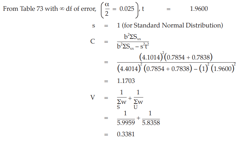
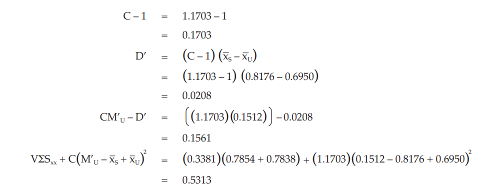
Calculate and apply ln confidence limits to ln potency ratio (M_L, M_U):

Confidence limits are given by antiln M_L and antiln M_U: antiln M_L = 0.8652 and antiln MU = 1.5793

Thus, the potency is estimated to be 163.80 IU/vial with confidence limits from 122.22 IU/vial to 232.54 IU/vial.

          If the precision of the assay is limited to be not less than 95.0 per cent and not more than 105.0 per cent of the estimated potency, the confidence limits of error will be 155.61 IU/vial and 171.99 IU/vial of the estimated potency.

Therefore, they do not imply such assay precision. The assay must be repeated and the combination of potency estimates is required.

3.2.4 The median effective dose

          In some types of assay it is desirable to determine a median effective dose which is the dose that produces a response in 50 per cent of the units. The probit method can be used to determine this median effective dose (ED₅₀), but since there is no need to express this dose relative to a standard, the formulae are slightly different.

(Note A standard can optionally be included in order to validate the assay. Usually the assay is considered valid if the calculated ED₅₀ of the standard is close enough to the assigned ED₅₀. What “close enough” in this context means depends on the requirements specified in the monograph).

         The tabulation of the responses to the test samples, and optionally a standard, and the test for linearity are as described in Example 11. A test for parallelism is not necessary for this type of assay. The ED₅₀ of test sample T, and similarly for the other samples, is obtained with the modifications as shown in Example 13. 

Example 13 The ED₅₀ Determination of a Substance Using the Probit Method, An in-vitro Assay of Oral Poliomyelitis Vaccine

In an ED₅₀ assay of oral poliomyelitis vaccine with 10 different dilutions in 8 replicates of 50 μl on an ELISAplate, results were obtained as shown in Table 58.

From Tables 59 to 66, the results are computerized and displayed as four decimal digits, without rounding off, except column (7).

Table 58 Dilutions of the Undiluted Vaccine

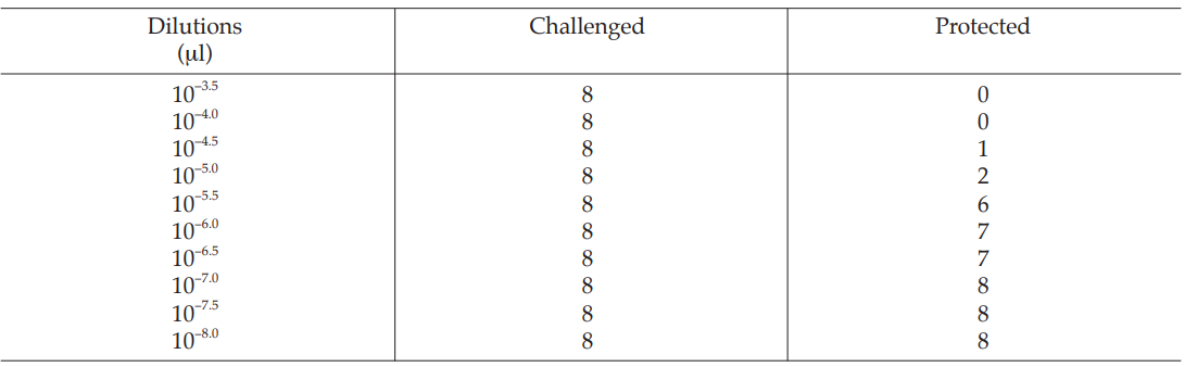
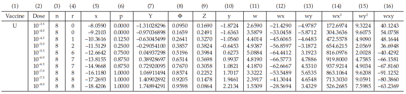
Table 59 First Working Table in the First Cycle

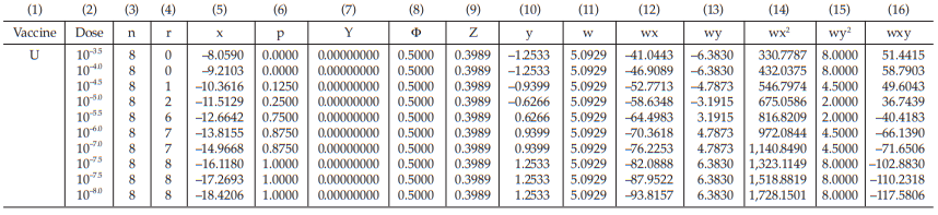
Table 60 Second Working Table in the Second Cycle

The data entered into the columns in the tables indicated by number:

(1) the vaccine label: U for test preparation,

(2) the dose of the standard or the test preparations,

(3) the number n of replicates for each treatment,

(4) the number of positive responding units r per treatment group,

(5) the natural logarithm of the dose, x,

(6) the fraction of positive responses per group, p = 

for Vaccine U dose 10^–5.0,                      p = 

   = 0.2500

 For the first cycle:

(7) column Y is filled with zeros,

(8) the cumulative standard normal distribution function, Φ = Φ (Y),

for Vaccine U dose 10^–5.0,                                  Φ = 0.5000

(9) the compute of Z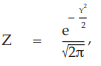                                                    

for Vaccine U dose 10^–5.0,                                  

= 0.3989

(10) the compute of y,                                                

for Vaccine U dose 10–5.0,                                

= –0.6266

(11) the compute of w                                                

for Vaccine U dose 10−5.0,                               

= 5.0929

The columns (12) to (16) in the first working table can be calculated from columns (5), (10) and (11) as wx, wy, wx² , wy² and wxy, respectively.

The sums calculated from columns (11) to (16) are transferred to columns (18) to (23) respectively.

(24) the compute of S_xx,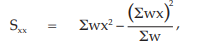                                                               

for Vaccine U,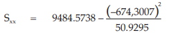                                                          

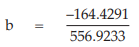
= 556.9233

(25) the compute of Sxy,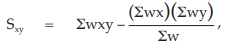                                                     

for Vaccine U,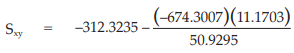                                                          

= –164.4291

(26) the compute of Syy,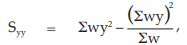                                                   

for Vaccine U,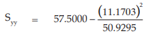                                                        

= 55.0500

(29) the compute of common b,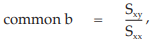                                           

= –0.2952

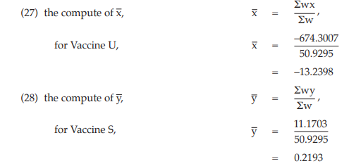
(30) the compute of a,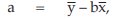                                                     

for Vaccine U,                                                        a = 0.2193 – (–0.2952)(–13.2398)

= –3.6896

Table 61 First Working Table in the Second Cycle

Table 62 Second Working Table in the Second Cycle

For the second cycle:

the column (7) of the first working table in the second cycle (Table 61) can be replaced by Y = a + bx (using a and b from the first cycle),

for Vaccine U dose 10–5.0 , Y = – 3.6896 + (–0.2952)(–11.5129) = – 0.2905

The next cycles are not show but they are repeated until the difference in Y between two consecutive cycles has become smaller than 10–8 .

Tables 63 and 64 show the cycle before sufficient and Tables 65 and 66 show the sufficient cycle.

The cycles shown in Tables 65 and 66 are sufficient for the estimation.

Table 63 First Working Table in the Cycle before Sufficient

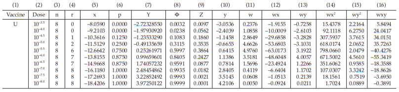
Table 64 Second Working Table in the Cycle before Sufficient

Table 65 First Working Table in the Sufficient Cycle

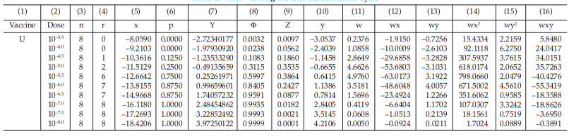
Table 66 Second Working Table in the Sufficient Cycle

Test of validity

Before calculating the potencies and confidence interval, test for linearity and parallelism of the assay must be assessed.

Test for linearity: 

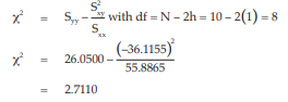
The χ2 with 8 degrees of freedom is 2.7110 representing a p-value of 0.9511 which is not significant deviations from linearity.

Estimation of potency and confidence limits

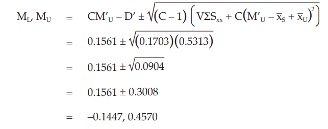
When there are no indications for a significant departure from linearity the ln (potency ratio), M’_U, is calculated as

Given statistic values for the next steps:

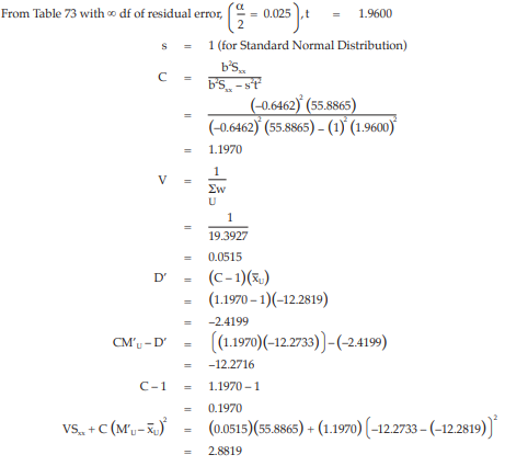
Calculate and apply ln confidence limits to ln potency ratio (M_L, M_U):

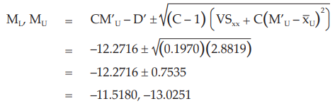
This estimate is still expressed in terms of the ln (dilutions). In order to obtain estimates expressed in ln (ED₅₀)/ ml the values are transformed to:

To express the potency of the vaccine in terms of log(ED₅₀)/ml, the results are divided by ln (10):

Confidence limits are given by M_L and M_U: M_L = 6.3032 log(ED50)/ml and M_U = 6.9577 log(ED₅₀)/ml

Thus, the potency is estimated to be 10^6.63 ED₅₀/ml with 95 per cent confidence limits from 10^6.30 and 10^6.96 ED₅₀/ml.

4. Combination of Assay Results

4.1 INTRODUCTION

          Replication of independent assays and combination of their results is often needed to fulfil the requirements of the Pharmacopoeia. The question then arises as to whether it is appropriate to combine the results of such assays and if so in what way.

          Two assays may be regarded as mutually independent when the execution of either does not affect the probabilities of the possible outcomes of the other. This implies that the random errors in all essential factors influencing the result (for example, dilutions of the standard and of the preparation to be examined, the sensitivity of the biological indicator) in one assay must be independent of the corresponding random errors in the other one. Assays on successive days using the original and retained dilutions of the standard therefore are not independent assays.

          There are several methods for combining the results of independent assays, the most theoretically acceptable being the most difficult to apply. Three simple, approximate methods are described below; others may be used provided the necessary conditions are fulfilled.

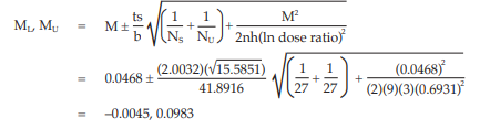
          Before potencies from assays based on the parallel-line or probit model are combined they must be expressed in logarithms; potencies derived from assays based on the slope-ratio model are used as such. As the former models are more common than those based on the slope-ratio model, the symbol M denoting ln potency is used in the formulae in this section; by reading R (slope-ratio) for M, the analyst may use the same formulae for potencies derived from assays based on the slope-ratio model. All estimates of potency must be corrected for the potency assigned to each preparation to be examined before they are combined.

          4.2 WEIGHTED AND UNWEIGHTED COMBINATIONS OF ASSAY RESULTS

          This method can be used provided the following conditions are fulfilled:

1) the potency estimates are derived from independent assays;

2) the number of degrees of freedom of the individual residual errors is not smaller than 6, but preferably larger than 15;

3) the individual potency estimates form a homogeneous set.

When the above conditions are met, the weighted mean potencies with confidence limits are calculated as described in Example 14.

          In case a significant variability between the assays exists and the individual potency estimates form a heterogeneous set. Under this circumstance condition 3 is not fulfilled and the method described in Example 14 is no longer applicable. The method described in Example 15 may be used.

          When these conditions are not fulfilled this method cannot be applied. The unweighted combination of assay results can be performed by the method described in Example 16 to obtain the best estimate of the mean potency to be adopted in further assays as an assumed potency.

Example 14 Weighted Combination of Assay Results, Homogeneous Set

          Six independent potency estimates of the sample preparation are described in Table 67. In Table 68, the results are computerized but only four decimal digits, without rounding off, are displayed.

Table 67 Potency Estimates and Confidence Intervals of Six Independent Assays

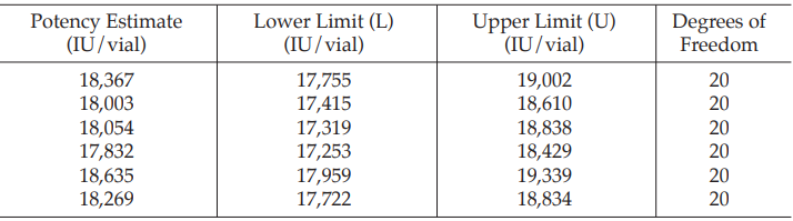
Table 68 Weighted Mean of Individual Assay Results

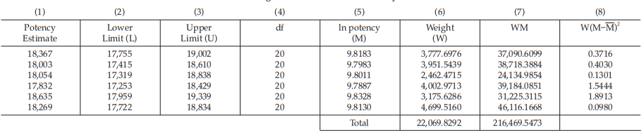
The data entered into the column in the tables indicated by number:

(1) the potency estimate,

(2) the lower limit of the estimated potency,

(3) the upper limit of the estimated potency,

(4) the number of degrees of freedom of their error variances,

(5) the natural logarithm of the potency, M,

Given statistic values for the next steps:

(6) the compute of W,               

for the potency estimate 18,367,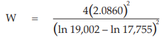

(7) the compute of WM for the potency estimates for the ln potency 9.8183, WM = (3,777.6976) (9.8183)

      = 37,090.6099

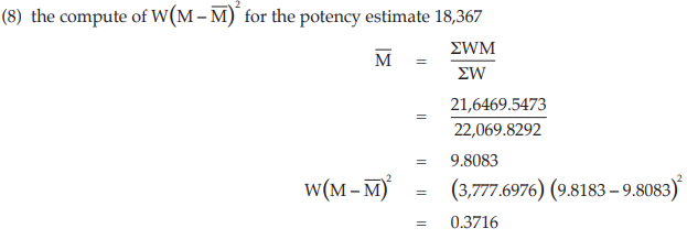
Test for homogeneity of potency estimate   

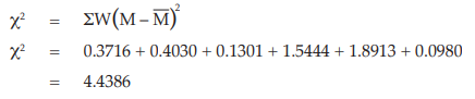
The calculated is χ2 smaller than the tabulated value corresponding to 5 degrees of freedom (11.070): the potencies are homogeneous.

Calculation of the weighted mean and confidence limits:

Given statistic values for the next steps:

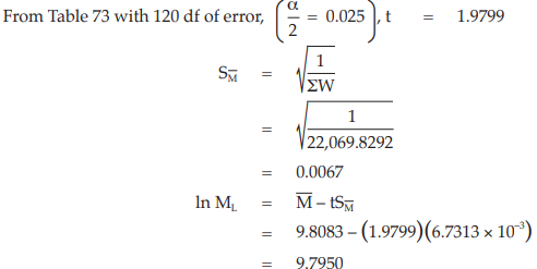
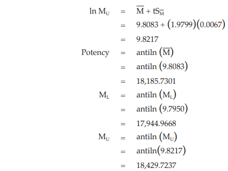
Thus, the potency is estimated to be 18,186 IU/vial with 95 per cent confidence limits from 17,945 to 18,430 IU/vial.

Example 15 Weighted Mean Confidence Limits based on the Intra-and Inter-assay Variation, Potency Estimates and Confidence Intervals of Six Independent Assays.

          Six independent potency estimates of the same preparation are described in Table 69. In Table 70, the results are computerized but only four decimal digits, without rounding off, are displayed.

Table 69 Potency Estimates and Confidence Intervals of Six Independent Assays

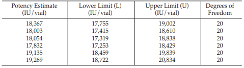
Table 70 Weighted Mean of Individual Assay Results

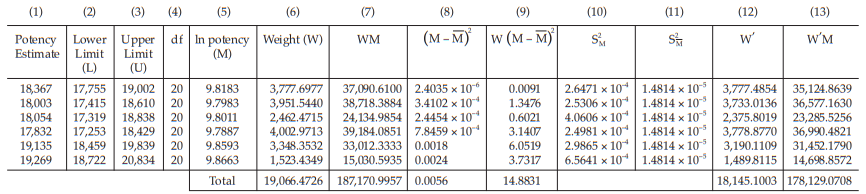
The data entered into the column in the tables indicated by number:

(1) the potency estimate,

(2) the lower limit of the estimated potency,

(3) the upper limit of the estimated potency,

(4) the number of degrees of freedom of their error variances,

(5) the natural logarithm of the potency, M,

Given statistic values for the next steps:

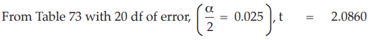
(6) the compute of W,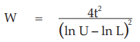                                               

for the potency estimate 18,054,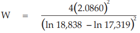                      

= 2,462.4715

(7) the compute of WM for the potency estimate

for the ln potency 9.8011,                                    WM = (2,462.4715) (9.8011)

= 24,134.9854

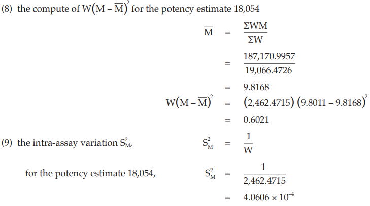
Given statistic value for the next steps:

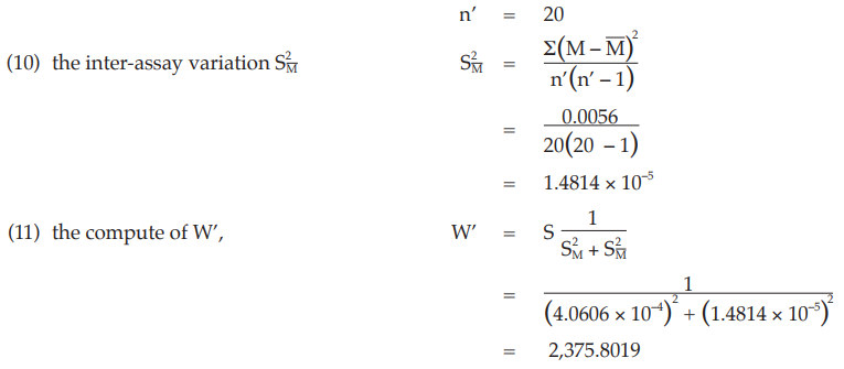
(12) the compute of W’M for the potency estimate 18054,

W’M = (2,375.8019)(9.8011)

       = 23,285.5256

Test for homogeneity of potency estimate

          By squaring the deviation of each value of M from the weighted mean, multiplying by the appropriate weight and summing overall assays, a statistic is obtained which is approximately distributed as χ² and which may be used to test the homogeneity of a set of ln potency estimates.

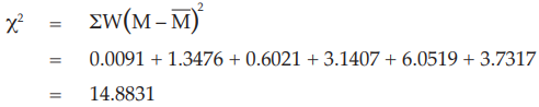
The calculated χ² is greater than the tabulated value corresponding to 5 degrees of freedom (11.070): the potencies are heterogeneous.

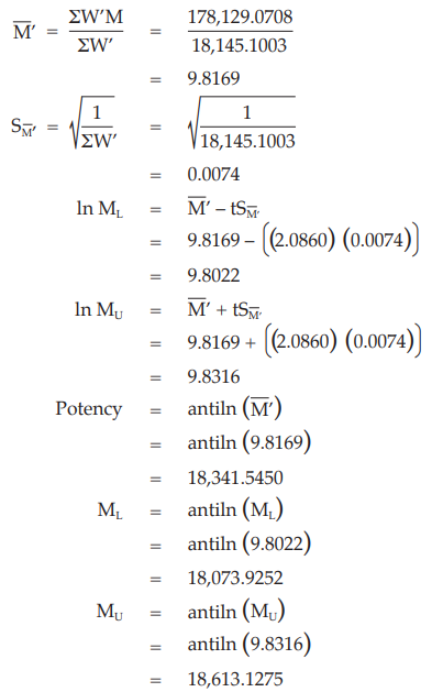
Thus, the potency is estimated to be 18,341 IU/vial with 95 per cent confidence limits from 18,073 to 18,613 IU/vial.

Example 16 Unweighted Combination of Assay Results

          Six independent potency estimates of the sample preparation are described in Table 71. In Table 72, the results are computerized but only four decimal digits, without rounding off, are displayed.

Table 71 Potency Estimates and Confidence Intervals of Six Independent Assays

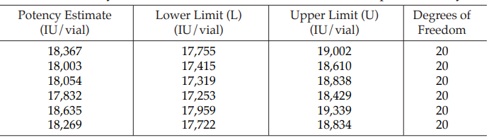
Table 72 Unweighted Mean of Individual Assay Results

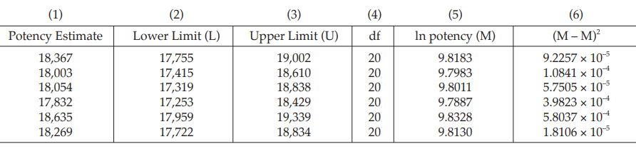
The data entered into the column in the tables indicated by number:

(1) the potency estimate,

(2) the lower limit of the estimated potency,

(3) the upper limit of the estimated potency,

(4) the number of degrees of freedom of their error variances,

(5) the natural logarithm of the potency, M,

Given statistic values for the next steps:

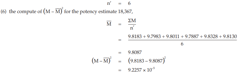
Calculation of the unweighted mean and confidence limits:

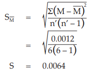
Given statistic values for the next steps:​

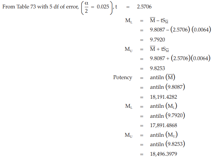
Thus, the potency is estimated to be 18,191 IU/vial with 95 per cent confidence limits from 17,891 to 18,496 IU/vial.

 

5. Table

          The tables in this section list the critical values for the most frequently occurring numbers of degrees of freedom. If a critical value is not listed, reference should be made to more extensive tables. Many computer programs include statistical functions and their use is recommended instead of the tables in this section. Alternatively, the generating procedures given below each table can be used to compute the probability corresponding to a given statistic and number of degrees of freedom.

Table 73 Upper Percentiles of the t-Distribution

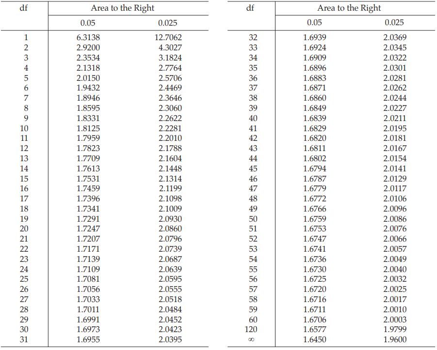
Table 74 Percentage Points of the Chi-Square Distribution* (χ² )​

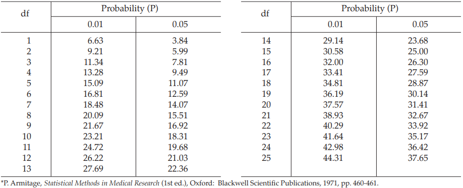
Table 75 Percentage Points of the F Distribution*​

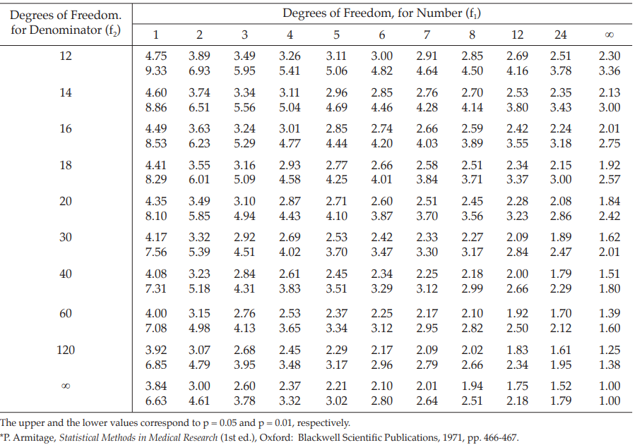
Table 76 The Φ − Distribution (the Cumulative Standard Normal Distribution)​

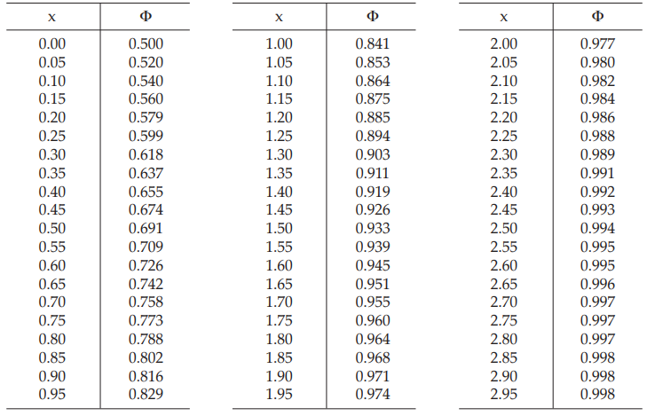
6. Glossary of Symbols​

SYMBOL	DEFINITION
a	Intersection of linear regression of responses on dose or ln (dose)
b	Estimate of slope of regression line of responses on dose or on ln (dose) based on all preparations in the assay
d	Number of dose levels for each preparation (excluding the blank in slope ratio assay)
df	Degrees of freedom
e	Base of natural logarithms (= 2.71828182845905...)
h	Number of preparations in an assay, including the standard preparation
n	Number of replicates for each treatment or number of blocks
p-value	Probability of a given statistic being larger than the observed value. Also used as the ratio r/n in probit analysis
r	The number of responding units per treatment group in assays depending upon quantal responses
s	Estimate of standard deviation
s2	Estimate of variance given by mean square of residual error in analysis of variance
si	Dose level of ith standard preparation (i = 1, ..., d)
sM	Estimate of standard deviation of log potency (M)
	The standard error of the mean potency
t	Student’s t-statistic
u	The ln (dose)-response function of four-parameter model
ui , zi	Dose level of ith unknown preparations U and Z (i = 1, ..., d)
y	Individual response or transformed response
F(cal)	Calculated variance ratio
F(tap)	Percentage Points of the F Distribution
L	Sum of linear contrasts
M	Estimate of In potency ratio
	The logarithm of the weighted mean potency.
N	Total number of responses in an assay (= hdn)
Q	Quadratic curvature sum of squares from analysis of variance
R	Estimated potency ratio of a given test preparation
S	Total response to a standard preparation
U,Z	Total responses to test preparations U and Z
W	Weighting factor in combination of assay results
Y	Vector representing the (transformed) responses in general linear models
Z	The first derivative of Φ
α	Level of significance, the given probability of a false rejection of the true null hypothesis in a statistical test
α’	Upper asymptote of the ln (dose)-response curve in four-parameter analysis
¶	3.141592653589793238...
Φ	Cumulative standard normal distribution function
χ2	Percentage Points of the Chi-square Distribution